GPU Accelerated Fourier Continuation Solvers and Physically Exact Computational Boundary Conditions for Wave Scattering Problems

(1)

physically exact computational boundary conditions

for wave scattering problems

Thesis by Tim Elling

In Partial Fulfillment of the Requirements for the Degree of

Doctor of Philosophy

California Institute of Technology Pasadena, California

2013

(2)

c

(3)

Acknowledgements

I owe a great debt of gratitude to Professor Oscar P. Bruno, who served not only as my advisor, but also as an excellent teacher, mentor, and friend. Over the past years he has shared with me his deep wisdom, great enthusiasm, and endless patience. Most importantly, he has always challenged my assumptions, not only of my work but also of myself. I would like to thank all of those whose help and support has made this thesis possible: Nathan Albin helped me with many discussions concerning the FC(Gram) method, and in particular its parallel implementation; David Hoch provided assistance to understand the details of the boundary condition work; Professor Tim Warburton graciously provided a specially modified version of his MIDG code for the hybrid solver, as well as his sage advice regarding the stability of time-domain methods in general. Edwin Jimenez helped me improve my mathematical writing, in particular in the preparation of this text. Conversations with Professor Catalin Turc both furthered my understanding of the equivalent source algorithm and encouraged my personal intellectual growth. I appreciate the continuous efforts of the various administrative staff at Caltech for their kindness and patience, in particular Sheila Shull, Sydney Garstang, and Carmen Sirois in the CMS department, and Tess Legaspi and Gloria Brewster in the registrar’s office. The specialized GPU implementations in this work would not have been possible without the help of our system administrators Chad Schmutzer and Will Yardley, who supported my many esoteric hardware and software requests.

(4)

and Herman Robinson for first introducing me to computers on his Apple ][+, which I still own today.

I would like to express my most profound gratitude to Christina Chow, my loving wife, without whose tireless support I may never have dared partake in this endeavor. Her boundless energy and encouragement have given me the drive needed to face the many late nights and long weekends that fueled this research.

(5)

Abstract

Many important engineering problems, ranging from antenna design to seismic imaging, require the numerical solution of problems of time-domain propagation and scattering of acoustic, electromagnetic, elastic waves, etc. These problems present several key difficul-ties, including numerical dispersion, the need for computational boundary conditions, and the extensive computational cost that arises from the extremely large number of unknowns that are often required for adequate spatial resolution of the underlying three-dimensional space. In this thesis a new class of numerical methods is developed. Based on the re-cently introduced Fourier continuation (FC) methodology (which eliminates the Gibbs phe-nomenon and thus facilitates accurate Fourier expansion of nonperiodic functions), these new methods enable fast spectral solution of wave propagation problems in the time do-main. In particular, unlike finite difference or finite element approaches, these methods are very nearly dispersionless—a highly desirable property indeed, which guarantees that fixed numbers of points per wavelength suffice to solve problems of arbitrarily large extent. This thesis further puts forth the mathematical and algorithmic elements necessary to pro-duce highly scalable implementations of these algorithms in challenging parallel computing environments—such as those arising in GPU architectures—while preserving their useful properties regarding convergence and dispersion.

(6)

case with the FC scattering solvers mentioned above, the boundary-conditions algorithm is modified into a formulation that admits efficient implementation in GPU and other parallel infrastructures.

(7)

Introduction

Many physical processes of considerable scientific and engineering importance, ranging from acoustics to electromagnetics, elasticity, and seismic phenomena, concern wave propagation and scattering. Acoustic scattering (deflection of pressure waves by particles or bodies in a medium) is the prototype for many of these physical processes. The precise mathemati-cal statement of wave interaction amounts to a system of conservation laws which is often formulated as a hyperbolic system of partial differential equations relating spatial and tem-poral derivatives of a perturbation in the underlying medium (in the case of acoustic waves) or in free space (in the case of electromagnetic waves).

(12)

with impedance boundary Γ, may be expressed in the form

1 c2

∂2

∂t2us−∆us=f(x, t) inR

3_\_Θ_×₍₀_,_∞) _(1.1) us(x,0) =u0(x) x∈R3\Θ (1.2) ∂

∂tus(x,0) = ˙u0(x) x∈R

3_\_Θ _(1.3) aus+bn· ∇us=−aui−bn· ∇ui (x, t)∈Γ×(0,∞) (1.4)

lim r→∞r

∂ ∂rus+

1 c

∂ ∂tus

= 0 r=kxk2, (1.5)

wheref(x, t) is a compactly supported source and the necessary initial conditions are given by u0(x) and ˙u0(x).

In order for the scattered field us to be uniquely determined it is necessary to require a certain condition of radiation at infinity (equation (1.5)) which was first introduced by Sommerfeld [70]. The direct scattering problem, then, is to determine this radiating solution us given knowledge of the partial differential equation, the incidence ui, and appropriate conditions (based on the physical properties under consideration) at the boundary of the scatterer(s). The numerical solution of exterior scattering problems poses unique challenges not present in bounded domains. Unbounded regions are usually truncated to render them suitable for numerical simulation, but doing so necessitates the specification of boundary conditions at the artificial boundary of the computational domain, which relate in subtle ways to the Sommerfeld radiation condition.

(13)

GPU execution, reducing the already-fast CPU boundary condition computing times by a factor of 50 on average in the GPU implementation, as shown in Section 9.3. Perhaps most importantly, this work provides the first efficient application of such an exact, radiating boundary condition to a nonconvex computational domain, and it in fact demonstrates a framework for the solution of multiple-scattering problems in Section 9.5 whose computing cost per time-stepremains independent of the distance between the scattering surfaces!

The remainder of this chapter presents a literature review on topics concerning the two main original contributions in this thesis, namely 1) Time-domain solvers for PDE prob-lems on unbounded domains by means of numerical algorithms on bounded computational regions, including a corresponding discussion of various numerical methods for evaluation of computational boundary conditions, (Section 1.1); as well as 2) Implementation in modern computing hardware leading to efficient, scalable methods for solution of computational science problems (Section 1.2).

1.1 Time domain methods and applications

1.1.1 Numerical PDE solvers

One of the oldest and best-known approaches for the numerical solution of time-domain wave propagation is the Yee scheme [78], also known as the finite-difference time-domain (FDTD) method. The FDTD scheme is appealing for its simplicity, and still sees broad commercial and scientific applicability, even though it is only accurate to second-order in both space and time. As is well known and evidenced, for example, in [20] (and shown in Section 9.1 of this thesis), a second-order FDTD method typically requires at least 96 pointsper wavelength, over a computational domain only 16 wavelengths across, in order to achieve a numerical accuracy of even 1%. Furthermore, as the acoustic size of the domain grows, the per-wavelength discretization must be increased in order to preserve accuracy, resulting in a requisite discretization that grows super-linearly with respect to the volume of the domain. Clearly, efficient solution of large scattering problems requires development of higher-order numerical methods. A thorough, modern accounting of the FDTD approach can be found in [74].

(14)

linear combinations of neighboring sample points on a regular lattice, with coefficients (or “stencil”) chosen in such a way that the truncation error, as evaluated through considera-tion of a relevant Taylor series expansion, tends to zero with a desired power of the mesh size. High-order FD schemes require increasingly wide stencils, posing difficulty near the boundary of the domain. So-called Pad´e or compact schemes, such as presented in [48, 61], partially alleviate this difficulty by posing an implicit equation for the derivatives, requiring solution of a banded linear system at each iteration. In either case, explicit or implicit FD, some accuracy is typically sacrificed near the computational boundary.

In order to model conservation laws directly, finite volume methods (FVM) [49], which are applicable to structured and unstructured meshes alike, produce the numerical solution via evaluation of numerical fluxes. By avoiding a formulation in terms of numerically-computed derivatives, FVMs are especially robust in the face of discontinuous solutions or “shocks”. Unfortunately, high-order convergence in FVMs is difficult to achieve, and often involves a nonlinear flux-limiter such as in [51].

The finite element method (FEM), within the broader class of Galerkin methods, replace the continuous PDE with a discrete weak-formulation. Originally developed for elliptic [63] and hyperbolic problems in diffusion, elasticity and structural analysis [77] and formalized in [72], this approach proceeds by dividing the computational domain into a number of geometric elements, over which the solution is represented as some linear combination of a set of piecewise-continuous basis functions. Perhaps the chief advantage of the FEM is its applicability to unstructured meshes, allowing for a broad class of computational domains to be discretized with relative ease. Evolving a time-dependent hyperbolic problem forward in time in some cases requires the solution of a sparse linear system at each time-step. Alternatively, the discontinuous Galerkin finite element methods [39] (DG-FEM) impose no conditions on the continuity between elements, allowing for an explicit update rule after the computation of a numerical flux term similar to that which appears in FVMs, at the expense of a greater number of numerical degrees of freedom.

(15)

spectrally-convergent and dispersionless solutions, but may only be applied to a highly re-strictive class of domains—most commonly rectangular parallelepipeds exhibiting periodic boundary conditions (possibly under even- or odd-extension). Chebyshev collocation meth-ods [10], on the other hand, either require stringent CFL conditions, due to refinement near the boundaries, or must be used in the context of implicit solvers, imposing the cost of solving a linear system every time-step.

1.1.2 Computational boundary conditions

For all of the numerical approaches discussed above, accurate treatment of an unbounded physical domain with a finite, bounded computational domain requires the specification of appropriate boundary conditions at the new (artificial) boundary. One famous approach, proposed first in [52] and later expanded in [26, 27], is applied in the form of a pseudo-differential operator based on increasingly accurate local approximations. This was later adapted in [57] for the case of electromagnetic waves. Similar local asymptotic approxima-tions generalizing this framework are presented by [8]. Another local boundary operator is proposed in [41] that is exact for plane waves traveling in a number of discrete directions. Yet another related approach described in [45] constructs a pseudodifferential operator that is perfectly absorbing for solutions traveling at a specified group velocity. One of the most broadly used methods today involves the construction of a “perfectly matched layer” (PML), first proposed for scattering problems in electromagnetism by [9]. This artificial layer acts as an absorbing media while producing minimal internal reflections, if the PML is taken to be sufficiently large. A more complete theoretical understanding of the PML was es-tablished in [21], and further improvements to the approach are developed in [22, 64]. The “complete radiation boundary condition”, or CRBC, is a recently introduced local method that reduces the impact of long-time errors on the solution is described in [36].

(16)

and later adapted by [37] to electromagnetics, the historical difficulty in this otherwise powerful approach lies in the costly evaluation of the integral representations of the solution, dominating the computational time of the interior solvers. A fast alternative based on Fourier and Laplace transforms was developed by [3, 4], but loses geometric generality, as it is only applicable to simple (e.g., spherical, cylindrical) computational domains, thus leading to very large unnecessary computational costs for problems for which the domain aspect ratio deviates significantly from one. Another efficient integro-differential approach was independently developed by [69] and [35], which is only applicable to spherical domains. In [65] a fast method based on Huygens’ principle and, more specifically, the presence of lacunae, solves an auxiliary system with the introduction of an inhomogeneity in a layer conforming to the computational boundary.

1.1.3 Numerical methods developed in this thesis

As mentioned in Section 1.1 and discussed in detail in Section 3.2.3, the most commonly used numerical PDE solvers for wave propagation problems suffer from significant loss of efficiency as the acoustical size of the computational domain is increased—owing to the lin-ear growth of the multiplicative constants in the algorithms error estimates with respect to the diameter of the domain; see equation (3.18) and Section 3.2.3. This phenomenon, which is caused by the underlying “dispersion error” (which is also known as “pollution error” in the finite-element context), is effectively resolved in the context of spectral methods such as the Fourier collocation and Chebyshev algorithms. The Fourier-continuation-(FC)-based PDE solvers [1, 18, 53] considered in this work, which are described in detail in Chapter 2, are spectrally accurate, and hence nearly dispersionless in the interior of the domain, but they are much more general than classical spectral methods: unlike the Fourier collocation method, the FC algorithms can be applied to general nonperiodic problems in general do-mains, and unlike the Chebyshev spectral methods, they do not entail highly restrictive Courant-Friedrichs-Lewy (CFL) time-step constraints. In this thesis, an FC-based numer-ical solver for the acoustic wave equation is introduced (Chapter 3), and it is hybridized with other numerical solvers (Chapter 8).

(17)

nonlocal methods potentially require the costly extension of the computational domain to a sphere. In these regards, this thesis extends the work of [42] (a fast method that can evaluate convergent, nonlocal boundary conditions) to cases that include nonconvex and even disjoint domains—a feature demonstrated for the first time in the present work (Sec-tion 9.5).

1.2 Parallel computing

Moore’s law has been a continual boon for all scientific fields that rely on numerical simula-tions. Originally presented in the 1965 paper [56], this “law” was an expression of the simple factual observation that the number of transistors available on each new generation of in-tegrated circuits appeared to be growing exponentially. Though the figure is not exact, the period over which these devices double in complexity (measured simply by transistor count) is often quoted to be 18 months [46]. What was once a rather casual observation, however, has become a self-fulfilling prophecy. For years now, Moore’s law has been a continually moving target that the semiconductor industry places on its own research and development efforts. Even though nearly 50 years have passed since Moore’s original publication, this trend continues today, and with the current technological horizon, is expected to continue for at least several years, possibly into the next decade [47].

Of far more interest to the mathematical community as consumers of computing tech-nology, however, is the implied performance. Fortunately this trend has also applied to measures of computational progress that, from the computational viewpoint, have far more practical interest—including available random access memory (RAM) and floating point op-erations per second (FLOPS). As an example, Intel’s original Pentium P5 architecture [44], introduced in March of 1993, could perform up to 75 MFLOPS, and it accommodated memory access at up to 554 MB/s. In contrast, November of 2008 saw the release of the first of Intel’s i7 line, the predominant architecture today, the first instance of which was the 965 Extreme Edition—which is capable of approximately 51.2 GFLOPS while reading memory at 27 GB/s. That is, over a span of 15 years, the floating point speed increased by a factor of roughly 680 (doubling more than nine times over), while the memory bandwidth increased by a factor of 47 (doubling more than five times).

(18)

and greatest on the market. While the potential for raw computational speed has increased, the requirements for harnessing the full extent of the available computing power have grown in complexity. There are two major areas where such developments have influenced this work. Firstly, there has been an increasing gap between the ability of a state of the art processor to access memory (MB/s) and the rate at which it can perform computation (FLOPS). If a computation requires a large amount of memory access relative to the number of floating point operations performed, then the practical increase in computing power over the last decade is significantly reduced. Notice that, from the release of the first Pentium to the i7, the comparative speedup between floating point and memory speeds differs by more than an order of magnitude. Furthermore, the i7 965 EE cannot read memory fast enough (at 4 bytes per single precision value) to meet the demands of its floating point capabilities, assuming every operation requires at least one newly fetched operand from memory (such as summation over an array).

Secondly, there has been an increasing trend, over roughly the past decade or so, towards multi- and many-core architectures. The i7 processor previously mentioned is only capable of reaching its peak performance of 51.2 GFLOPS when a considerable degree of parallelism has been accounted for, taking advantage of all four cores in addition to using vectorized floating point operations (SSE) on each. If these considerations are neglected, the same device would only be capable of roughly 3.2 GFLOPS. This second difficulty is of even greater concern after noting that not every computation can be efficiently parallelized. Amdahl’s law [5] states no amount of parallelism can ever accelerate a computation beyond the time required for the longest purely sequential subcomputation. A formal (and slightly more general) statement is that, given a set of atomic computational tasks and the partial ordering implied by their dependencies, the minimal time to complete the computation is the largest sum of task times over any subset for which the partial ordering implies a unique full ordering. Algorithms that do scale well in this domain, in part by minimizing this property, will be of ever-greater importance as this trend continues.

1.2.1 Shared and distributed memory environments

(19)

com-munication between them. The most widespread (but not only) model for programming in such an environment is the message-passing model, the most famous implementations thereof adhering to the message passing interface (MPI) standard [68], in which a separate copy of the program is run on each node, with interdependencies in the computation man-aged by the passing of messages, either point to point (matched send and receive pairs) or collective group communications (such as broadcast and parallel reductions). In order to efficiently use such a device, there are two concerns that are typically addressed: the amount of computational work for which each node is responsible should be reasonably balanced, and the cost of communication incurred by distributing said work should be limited.

This is in contrast to the less-scalable but simpler “shared memory” model, where a single program is split into several parallel “threads”, each having direct access to the same physical memory. Two of the most common APIs for this style of development are POSIX-threads, for which the manual creation and management of each computational thread is necessary, and OpenMP [24], which abstracts this work into a much cleaner interface, but is only well-supported by more recent compilers and tools. Shared memory models have the advantage of greatly reducing the cost of communication, but place a greater burden on the programmer to ensure program correctness (thread safety). Furthermore, while most modern desktop computers naturally support this style of parallelism, the cost of shared memory hardware tends to grow much faster, as a function of the number of cores, than the cost of a comparable distributed memory system, and even still necessarily sacrifices some memory performance owing to purely physical limitations in their construction.

(20)

1.2.2 General purpose graphics processing units

Modern GPUs are an extreme case of the many-core engineering trend. Originally designed as specialized hardware to perform a fixed number of simple functions on a pixel or per-texel basis, current-generation GPUs are fully programmable and often feature a number of cores totaling in the hundreds. Each of these cores, however, is far more limited in functionality than the corresponding cores of a traditional desktop CPU.

NVIDIA Corporation’s Compute Unified Device Architecture (CUDA) provides a pro-gramming model [59] specifically for these modern many-core programmable GPUs. CUDA provides both an abstraction of the underlying hardware and its capabilities, as well as a programming environment (CUDA for C) for developing applications. In the CUDA model, a single GPU is comprised of a uniform global memory space plus a number of symmetric multiprocessors (SMPs). Each SMP possesses a number of parallel computing cores called streaming processors (SPs), which collectively share a small pool of local memory and a

single instruction unit—a detail of great importance, since even though an SMP on a typical GPU may have 16 SPs, they must all execute identical instructions in lock-step. This results in what NVIDIA has dubbed the “single-instruction, multiple-thread” or “SIMT” execu-tion model, whose nomenclature follows from “single-instrucexecu-tion, multiple-data” (SIMD) and similar designations. For simplicity, a collection of threads running in parallel, over identical instructions, on an SMP is referred to as a “threadblock”.

Following the SIMT architecture, the second major deviation from standard CPU ar-chitectures is the manner in which memory is accessed. Each SMP possesses a single high-bandwidth, but high-latency, connection to global GPU memory. Furthermore, the memory caching mechanisms present on typical desktop CPUs to hide this physically nec-essary latency are conspicuously absent, requiring a developer to explicitly manage these delays, most importantly through a form of thread multiplexing discussed in more detail in Section 4.1. Finally, since an SMP may only access global GPU memory by reading or writing a 16-, 32-, or 64-byte contiguous block at a time, the underlying SPs must have their memory access patterns planned out in such a way that they collectively “coalesce” into these block operations, or else performance may be (quite literally) decimated.

(21)

architecture [66] (now superseded by the Intel many integrated core (MIC) architecture). They also provide, effectively, a snapshot into the anticipated future, with respect to relative floating point versus memory performance. In targeting these devices for development, then, one not only uses the most powerful floating-point devices currently available, but also potentially gains a leg-up on the architectural trends of the future.

1.2.3 Limited precision arithmetic

(22)

Chapter 2

Fourier continuation

Fourier collocation methods take advantage of the rapid convergence of Fourier series for smooth, periodic functions in order to enable the numerical solution of suitable problems in a manner that is both very accurate and efficient. Once a discrete function is expanded in a Fourier basis, common numerical operations such as differentiation become simple to imple-ment (as a diagonal operator) and yield spectral convergence. When solving time-dependent partial differential equations, spurious high-frequency oscillations associated with nonlin-earity or instability in the numerical solution may also be damped directly in a manner analogous to the introduction of artificial viscosity, improving the stability of such methods without significantly impairing the numerical accuracy and without greatly increasing nu-merical dispersion. Furthermore, the fast Fourier transform [23] (FFT) provides an efficient means of mapping a function to and from the discrete Fourier basis in only O(NlogN) time. The limitation of the Fourier collocation methods, however, is that the PDE solution must be a periodic function over a rectangular domain: if the Fourier collocation method is applied to a nonperiodic function directly, the resulting representation converges very poorly, with slow convergence in the domain interior, and with an O(1) error near the boundary. In other words, if Fourier collocation is used for nonperiodic functions, then the Gibbs phenomenon takes place. The Fourier continuation method provides a means to ad-dress this difficulty, and thus enables spectral treatment of PDE problems whose solutions are not periodic functions.

(23)

intro-duce the Fourier continuation method, consider a given (generically nonperiodic) function f : [0,1]→_C, defined in the interval [0,1], whose discrete samples

fn=f(xn), xn= n

N−1, n= 0. . . N −1 (2.1)

are known. In order to represent the functionf by a Fourier series while avoiding the Gibbs phenomenon, a Fourier expansion of f is sought on an interval [0, b] withb > 1. That is, the Fourier continuation method seeks to produce a function fc of the form

fc(x) = W

X

k=−W cke2πi

kx

b (2.2)

which agrees with f as closely as possible, in the in the interval [0,1] where f is defined. The functionfcsmoothly transitions over the interval [1, b] to create ab-periodic extension, as depicted in Figure 2.1 for the particular case of the functionf(x) =x. Unfortunately, it is no longer possible to directly compute the coefficientsck, offcwith a simple application of an FFT. The remainder of this chapter discusses two methods for the construction of such expansions, including an FFT-based algorithm with a cost essentially identical to that of a single FFT.

2.1 Fourier continuation based on singular value

decomposi-tion

The most direct (if not the most efficient or best conditioned) approach for the determination of the Fourier series coefficients ck results [11, 15, 19] as the N known data points together with the definition of fc_{are interpreted as a system of}_N _{equations for}_M _unknowns:

fn= W

X

k=−W cke2πi

kxn

b . (2.3)

(24)

0 0.5 1 1.5 2 −0.5

0 0.5 1 1.5

x

[image:24.612.155.492.70.359.2]

fc(x) f(x)

Figure 2.1: Fourier continuation fc(x) of the function f(x) =x

the present discussion may prove useful nevertheless.) Defining the matrix A by1:

Amn =



 

 

e2πimxnb when m≤W

e2πi(W −m)xn

b otherwise,

(2.4)

the desired coefficients ck are then given by the components of the solution vector y of the problem

min

y kAy−bk2, (2.5)

wherebn=fn. The singular value decomposition [33]

A=U SVH (2.6)

(whereU, V are unitary matrices and whereSis a nonnegative diagonal matrix) is a natural choice for the solution of least-squares problems of this type. Defining the pseudo-inverse S+of the diagonal matrixSas the diagonal max(M, N)×max(M, N) matrix whose nonzero

1

(25)

elements equal the reciprocals of the corresponding nonzero elements of S, in terms of this decomposition the least solutiony is given by

y=V S+UHb. (2.7)

The least-squares problem just considered becomes ill conditioned as N and/or M are increased—in light of which, it is necessary to use a truncated pseudoinverse ofS,S+, that is, a diagonal matrix with coefficients defined by

(S+)mm=

  

 

(Smm)−1 when Smm

S0,0 ≥

0 otherwise.

(2.8)

The parameteris typically taken to be on the order of machine precision. As demonstrated by [15], this method converges to order r−1 provided thatf(x)∈Cr.

As mentioned above, this approach is computationally expensive and ill conditioned. Indeed, evaluation of the singular value decomposition requires O(M N2+N3) operations, and solution of the system (per set of unknowns, once the SVD is available) requiresO(M2+ M N) operations. Although in the surface representation context [15] these issues do not pose significant difficulties, the application of this approach to the solution of time-domain PDEs would give rise to a prohibitively expensive solver. Furthermore, the ill-conditioning inherent in the solution of the least-squares problem would limit severely the size of the problems that could be considered. Both of these difficulties are eliminated in the Fourier continuation algorithm presented in the following section.

2.2 Accelerated Fourier continuation based on Gram

poly-nomials

(26)

The main idea underlying the evaluation of theCextension values involves consideration of the function f(x), defined in the original interval [0,1], along with its translation by distance b,f(x−b), as implied by the fact that ab-periodic extension is desired. Selecting a positive integerdthat prescribes a certain number of “matched point-values” (the length of the interval where matching takes place is given by δ = (d−1)h) consider the set of d right-most discretization points in the interval [0,1], namely D_right = {xN−d, . . . , xN−1} as well as the set of d left-most discretization points Dleft = {b+x0, . . . , b+xd−1} in the interval [b, b+ 1]; see, e.g., Figure 2.2. Roughly speaking, the additionalC needed function values in the interval [1, b] are obtained as the point values of an auxiliary trigonometric polynomial, with periodicity interval [1−δ,2b−(1−δ)] and with appropriately selected bandwidth, produced by means of an FC(SVD) fit to the function values on Dright∪ Dleft, as described in what follows.

Polynomial interpolation of the function values on Dright ∪ Dleft is produced by means of two Gram (orthonormal) polynomial bases B_right and B_left of the respective spaces of polynomials of degree < don the intervals [1−δ,1] and [b, b+δ] and associated orthogonal projections. (The setsB_right and B_left are orthonormal bases of the space of polynomials of degree < dwith respect to the natural discrete scalar product defined by the discretization points D_right and D_left, respectively.) The algorithm then proceeds by precomputing, for each polynomial p ∈ Bright, a smooth function defined for x ≥ 1−δ, which approximates p closely in the matching interval [1−δ,1], and which blends smoothly to zero for x ≥b. Such rightward extension is obtained by means of appropriately oversampled least-squares approximations by Fourier series of periodicity interval [1−δ, b−(1−δ)], as described in [1]. Similarly, the scheme obtains, for each polynomial p ∈ Bright a smooth blending function that agrees withp in the matching interval [b, b+δ] and vanishes forx≤1.

(27)

fj augmented by the C additional “continuation” values fext just constructed yields the desired trigonometric continuation polynomial.

0 0.2 0.4 0.6 0.8 1 1.2 1.4 1.6

0 1 2 3 4 5 6 7

x

f(x) f

left

f

right

f

[image:27.612.146.497.123.415.2]

match

Figure 2.2: The function f(x) =esin(5.4πx−2.7π)−cos(2πx), sampled at N = 92 evenly spaced points over the intervalx∈[0,1], and its continuation via FC(Gram), usingd= 5 matching points and C = 25 extension points. The periodic continuation is superimposed to the right.

The operator that extends N given function values into N +C samples of a smooth periodic function is a sparse matrix operator with simple structure, composed of theN×N identity matrix and two smallC×dsubmatrices. The action of the extension operator can be expressed in the block-matrix form

˜ f =





IN

A



f = 



f

Af



, (2.9)

(28)

and last dcolumns. Using the notation

fl = (f0, . . . , fd−1)T, fr= (fN−d, . . . , fN−1)T, (2.10)

the vectorAf has the form

Af =AlQTl fl+ArQTrfr. (2.11)

Here, each column of Ql and Qr contain the dpoint values of one of the elements of the polynomial basis, and the columns of Al and Ar contain the C point values that blend the corresponding polynomials to zero, toward the left and right, respectively. As described above, when the left and right blending functions are added, theCneeded extension function values result. Because each of these are small, fixed matrices that can easily be precomputed, the application of the extension operator (2.11) can be performed very rapidly. By applying the FFT to the extended vector of function values ˜f the discrete coefficientsck are obtained and thus the desired representation (2.2) results.

The matrices Ar and Al differ only by row-ordering, and similarly, Qr and Ql only differ by column-ordering. As a consequence of this fact, only half as much data needs be stored/loaded as compared to the original presentation in the FC-AD work [18]. That is, definingRmas anm×mmatrix with ones on the antidiagonal, serving to reverse the order of elements in anm-vector under multiplication, the composition of matricesAlQl may be alternatively computed using

AlQl=RCArQrRd. (2.12)

(29)

2.3 Numerical differentiation

Once a convergent Fourier series representation of a function is obtained, the corresponding numerical derivative of the discrete series may be computed directly.

fc(x) = X m∈K

cme2πi

mx

b (2.13)

f_xc(x) = X m∈K

2πim bcme

2πimx_b _(2.14)

This can equivalently be seen as a diagonal operator applied to the Fourier coefficients, taking each cm to 2πim_b cm. Once the coefficients have been scaled by this complex factor, they may be inverted in O(NlogN) time via an inverse FFT, and finally restricted to the originalN discretization points. The discrete FC differential operator, then, is implemented as the following sequence of operations:

1. Expand the leftmost d and rightmost d values of f in the Gram polynomial bases Bright and Bleft, forO(d2) operations.

2. Sum the precomputed Gram polynomial extensions in the interval [1, b],O(Cd) oper-ations.

3. Compute the FFT of ˜f,O((N +C) log(N+C)) operations.

4. Differentiate the Fourier coefficients, O(N +C) operations.

5. Invert the FFT,O((N+C) log(N +C)) operations.

This algorithm has an overall the cost of orderO(d2+Cd+ (N+C) log(N+C)), which is dominated by the favorable scaling of the requisite FFTs.

2.3.1 Data filtering

(30)

by applying a scaling factor to the Fourier coefficients that dampen the contribution of higher-frequency terms. Given the finite series expansion

fc(x) =

X

ckeikx, (2.15)

the smoothed approximation is defined by

f_cσ(x) =Xσ(2k N)cke

ikx _(2.16)

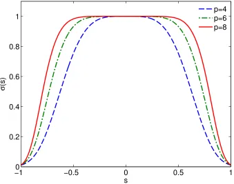
for a suitable function σ(s), defined over the normalized range of frequenciess∈[−1,1]. It was observed in [1] that the spectral filter

σ(s) =e−α|s|p, (2.17) discussed also in [38] and displayed in Figure 2.3, is particularly well suited to explicit time-domain solvers built using the FC(Gram) method. In [1] the parameterα is chosen to roughly equal −lnmachine (where machine is the “machine epsilon” [71]) in order to make the coefficients effectively vanish for |s|= 1, and pis taken to grow linearly with N, which results in a spectrally accurate filter. In the context of this work, however, it is found that a different choice of filter parameters is appropriate. The precise reasons for this, as well as the particular selection of values that prove to be useful, are presented in Chapter 4.

(31)

−10 −0.5 0 0.5 1 0.2

0.4 0.6 0.8 1

s

σ

(s)

[image:31.612.157.496.245.512.2]

p=4 p=6 p=8

(32)

Part II

Hyperbolic solver for bounded

(33)

Chapter 3

One-dimensional solvers

This chapter focuses on the spatially one-dimensional version of the types of problems under consideration in this thesis. Under this greatly simplified setting an FC-based method-of-lines is introduced, its stability and accuracy are studied, and its efficiency is compared with those of other available high-order solvers. Additional comparisons of the FC one-dimensional solver are presented in sections 4.2.2 and 9.1. The full three-one-dimensional solver is introduced in Chapter 5 and demonstrated in Chapter 9.

3.1 First-order hyperbolic systems

Hyperbolic equations characterize “wave-like” phenomena. Formally, a PDE is hyperbolic if the Cauchy initial value problem is locally solvable in the neighborhood of an arbitrary, noncharacteristic initial surface [29]. A linear hyperbolic PDE may, by the introduction of a sufficient number of auxiliary unknowns, be re-expressed as a first-order hyperbolicsystem. In one dimension, these systems for a vector unknown u(x, t) take the form

ut+A(x, t)ux=f(x, t) (3.1)

for some everywhere-diagonalizable matrix A(x) and inhomogeneityf(x, t).

(34)

discretiza-tions minimize the restricdiscretiza-tions imposed by the CFL condition. Unless otherwise stated, for all of the examples in this chapter the domain is the unit interval [0,1]: a problem on any other bounded interval is reduced to the interval [0,1] by an affine change of variables. The sample points are then

xn=nh, h= 1

N −1, n= 0. . . N −1; (3.2)

the corresponding function values at time t= tm will be denoted by umn ≈u(xn, tm). (In the event that the domain under consideration is periodic the mesh size h = _N1₋₂ is used instead, in order to avoid the prescription of a redundant sample point.)

Of the possible methods for time integration, the explicit Runge-Kutta and Adams-Bashforth methods [71], both of orders three and four, are of particular interest in the context of this thesis. The region of absolute stability for all four of these methods includes a symmetric interval, around the origin, along the imaginary axis. This is especially helpful for the class of problems discussed in this thesis. (In the case of the one-dimensional wave equation on a bounded domain, with typical (Dirichlet or Neumann) boundary conditions, for example, the eigenvalues ofA(x) are strictly imaginary.)

In order to accommodate nontrivial computational boundary conditions that may take the form of an ODE in time at the boundary, such as those discussed in Chapter 6, it is desirable to avoid the additional complexity introduced by the intermediate steps of the Runge-Kutta methods. Therefore the method of choice for time integration will be the Adams-Bashforth method, of order four (AB-4). It is necessary to initialize the first several steps of the method—but this is typically inconsequential, as these scattering problems normally have initial conditions of zero throughout the domain.

3.1.1 Advection equation

The simplest hyperbolic system is the linear advection equation for the scalar unknown u=u(x, t),

ut+cux = 0, (3.3)

(35)

hyperbolic systems in arbitrary spatial dimensions. Boundary conditions for hyperbolic problems are required wherever the characteristic curves enter the domain. Without loss of generality, in what follows it is assumed thatc >0.

3.1.2 Wave equation

The most common second-order form of the one-dimensional wave equation,

utt+c2uxx = 0 u(x,0) = f(x)

ut(x,0) = g(x),

is not expressed in the standard form of a first-order hyperbolic system. It is readily verified, however, that this equation is equivalent to the system

  u v   t +  

0 −c

−c 0

    u v   x

= 0 (3.4)

with the corresponding initial condition onv

v(x,0) =

Z 1

0

g(s)ds+ const. (3.5)

With an appropriate normalization, the unknowns u and v in this system correspond to pressure and velocity, respectively.

3.2 Accuracy, stability, and dispersion

(36)

presently under consideration stability will be demonstrated over a wide range of parame-ters, and the corresponding CFL condition and Courant number of the algorithm will be found. Finally, the near-dispersionless character of the method will be demonstrated by examining the performance of the algorithm as the size of spatial domain and the corre-sponding final solution time are dramatically increased while using a fixed number of sample points per wavelength.

3.2.1 Advection equation

Consider first the advection problem (3.3), and take zero initial conditions, in conjunction with the boundary condition

u(0, t) =e−a(t−0.5))2

where the parametera=−4 ln 10−16is chosen such that the function vanishes, to numerical precision, at t= 0. This problem admits the exact solution

u(x, t) =e−a(t−x−0.5)2.

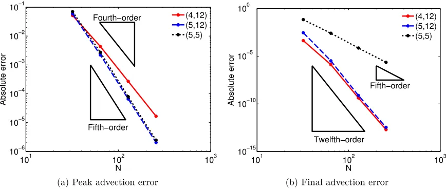
As part of this work it was found experimentally, in agreement with the conclusions presented in [1, 53], that dleft ≤ 5 must be used in order to ensure numerical stability where the physical boundary condition is applied. On the other hand, at the free right-side boundary, it is possible to selectdright = 12. This does not improve the overall order of the scheme in this case, since the left-side boundary still contributes a lower-order error, but it does offer some advantage, as will be shown below.

(37)

0 0.2 0.4 0.6 0.8 1 0

0.2 0.4 0.6 0.8 1 1.2

x

u

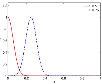
[image:37.612.160.496.72.349.2]

t=0.5 t=0.75

Figure 3.1: Advecting Gaussian

of a higher-order matching polynomial at the right-side boundary clearly distinguishes itself in Figure 3.2(b), even though the formal order of accuracy is not improved, as is seen in Figure 3.2(a) (though the error does decrease slightly as well).

To determine the CFL condition numerically, the solver may be run for many different discretizations in both space and time so that a consistent CFL relationship of the

µ= ∆t

∆x ≤C (3.6)

(38)

101 102 103 10−6 10−5 10−4 10−3 10−2 10−1 N Absolute error Fourth−order Fifth−order (4,12) (5,12) (5,5)

(a) Peak advection error

101 102 103

10−15 10−10 10−5 100 N Absolute error Fifth−order Twelfth−order (4,12) (5,12) (5,5)

[image:38.612.115.549.83.267.2]

(b) Final advection error

Figure 3.2: Spatial convergence of the 1d advection solver for various values of the order (dleft, dright)

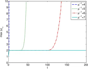
comprehensive testing of solution space with one, or a few, code runs.) If the solution, then, remains comfortably bounded for a very large number (typically millions to hundreds of millions) of time-steps, it can be inferred that the method is stable insofar as any practical application is concerned. In Figure 3.3 the error as a function of time is shown for several choices of µ. These few examples suggest C ≈ 1

7, which has been tested extensively, for many values of N, all run for millions of time-steps with random initial data.

In order to study convergence with respect to time, on the other hand, a spatially periodic configuration is considered—since for such a configuration the accuracy the of FC solver is particularly high, and, thus, the need for fine spatial meshes (which, in view of the CFL constraint, would prevent consideration of the larger time-steps in a time-convergence analysis) is minimized. For this convergence test the advection equation in the interval [0,1] was considered, with the initial condition

u(x,0) =e−a(x−0.5)2

and with the periodic boundary conditions

u(n)(0, t) =u(n)(1, t), n= 0,1. (3.7)

(39)

bound-0 0.5 1 1.5 2 2.5 3 0

0.2 0.4 0.6 0.8 1 1.2 1.4 1.6 1.8 2

t

|u|

∞

µ−1=4

µ−1=5

µ−1=6

[image:39.612.155.494.73.345.2]

µ−1=7

Figure 3.3: Maximum norm over time of the FC numerical solution of the advection equation the for several values of the parameter µ= _∆x∆t. Forµ−1= 7 the solution remains bounded indefinitely.

ary conditions such as (3.7) implicitly, by extending the discrete mesh points xn = nh to include a number df of additional points

{x−df, x−df+1, . . . , x0, . . . , xN−1, . . . , xN−1+df}

which, reaching past each one of the two boundary points, are also used as solution sampling points. The additional “fringe” points (namelyx−df, . . . , x−1andxN, . . . , xN−1+df) do not,

however, correspond to additional unknowns in the numerical system—instead, the function values at the fringe points are prescribed to equal the function values at the corresponding image points within the domain [0,1); for example, u−df = uN−df. This is equivalently

(40)

periodic operator ˜FM is defined by

˜ FM =

0 IM 0

FM+2df



   

0 Idf

IM

Idf 0

     . (3.8)

In order to demonstrate the convergence over a large range of discretizations in time, the spatial discretization is also refined, maintaining a fixed ratioµ= 1/8. Figure 3.4 shows the resulting convergence using AB-3 and AB-4, where in both cases the error is clearly dominated by the order of the time integration scheme.

102 103 104

10−8 10−6 10−4 10−2

Timesteps

Absolute error _{Fourth−order}

Third−order

AB−3 AB−4

(a) One period

103 104 105

10−8 10−6 10−4 10−2 100 Timesteps

Absolute error Fourth−order

Third−order

AB−3 AB−4

[image:40.612.112.549.277.461.2]

(b) Ten periods

Figure 3.4: Temporal convergence of 1d advection solver

Remark 3.2.2. The application of the FC method to a periodic domain (which is clearly unnecessary since the full Fourier collocation method could be utilized instead) is only used, here and later in this thesis, to demonstrate the behavior of the FC method under very controlled settings. It is worth pointing out, however, that the FC method in this context does not take advantage of the [0,1]-periodicity—since, indeed, it uses a periodicity interval larger than 1.

3.2.2 Acoustics

(41)

Dirichlet boundary conditions

u(0, t) =u(1, t) = 0

and with initial conditions given by

u(x,0) = e−a(x−0.5)2

v(x,0) = −e−a(x−0.5)2.

Note that these initial conditions specify a right-moving wave packet much like the one used in the advection example of the previous section. In fact, by taking the periodic extension

G(x) = ∞

X

n=−∞

χ_[0,1](x+ 2n)e−a(x+2n−0.5)2,

where χ_[0,1] denotes the characteristic function of the interval [0,1], the exact solution for all time can be expressed in closed form

u(x, t) = G(x−t)−G(x+t−1)

v(x, t) = G(x+t−1)−G(x−t).

Boundary conditions may be applied on any linear combination ofuandvthat contains a component in the direction of the incoming characteristic derivative. The boundary condition here is applied to u only, while the corresponding boundary values of v remain free variables in the system. In order to ensure stability two steps were taken, namely 1) The degree of the matching Gram polynomials were restricted at the physical boundaries, but now at both ends of the domain, as well as for both unknowns; and 2) The exponential filter (2.16) introduced in the previous chapter was used. This filter is applied twice at each time-step: once as part of the numerical differentiation, and again, independently, to the solution unknowns. The overall filtered explicitr-step time integration scheme with weights wj can be expressed in the form

un+1=Iσun+ ∆t r−1

X

j=0

wjDσun−j, (3.9)

(42)

the unfiltered Adams-Bashforth methods, this operator would simply be the identity). An important observation is that, since the matrices Iσ and Dσ do not necessarily commute, the traditional stability criterion (root condition) for the Adams-Bashforth methods does not apply, at least not exactly. With this caveat, however, the root condition remains a goodindicator of stability, whose predictions can be once again verified via comprehensive numerical studies.

Figure 3.5 demonstrates that, in absence of the exponential filter mentioned above, spurious oscillations in the numerical solution occur. As shown in Figure 3.6, in contrast,

0 0.2 0.4 0.6 0.8 1

−1 −0.5 0 0.5 1

x

Solution

u v

(a) Solution at timet= 1.

0 0.2 0.4 0.6 0.8 1

−10 −5 0 5 10 15

x

Solution

u v

(b) Solution at timet= 1.5.

Figure 3.5: Instability of the unfiltered FC wave-equation solver at two different points in time. The problem was discretized using N = 54 points in space. Att= 1 the instability is visible, as it first occurs, and byt= 1.5 it strongly dominates the true solution.

the filtered algorithm is stable provided a CFL condition is satisfied. The filter parameters

p= 8 and α=−8µln 10−2 (3.10)

are used here and elsewhere in this thesis—whenever the exponential filter is applied. This is notably different from the typical usage of this filter as described in [38], since the coeffi-cients do not numerically vanish for the highest frequency modes. On the other hand, this selection is entirely sufficient to ensure stability for the solvers considered in this thesis, and furthermore, it is a closer approximation of the identity operator. The resulting method has Courant number roughly C≈ 1₇, as is demonstrated in Figure 3.6.

(43)

0 50 100 150 200 0

1 2 3 4 5 6 7 8 9 10

[image:43.612.155.492.77.345.2]

t

max |u|

∞

µ−1=4

µ−1=5

µ−1=6

µ−1=7

Figure 3.6: Maximum norm of the computed solution of the wave equation (in first-order system form) for several values of the parameter µ = _∆x∆t, using a frequency domain filter withp= 8 and a=−ln 10−2

those presented in Section 3.2.1 for the advection equation, are presented here in Figure 3.7. The present error curves replicate almostexactly those presented earlier for the advection equation with matching polynomials of degrees dleft=dright = 5.

(44)

102 103 10−8 10−6 10−4 10−2 100 N

Absolute error Fifth−order

Fourth−order

d=4 d=5

(a) Spatial convergence.

102 103 104

10−8 10−6 10−4 10−2 100 Timesteps Absolute error Fourth−order Third−order AB−3 AB−4

(b) Temporal convergence.

Figure 3.7: Convergence of the numerical solution of the wave equation in first-order system form; cf. the corresponding graphs presented in Figures 3.2 and 3.4 for the advection equation.

3.2.3 Dispersion

One of the greatest strengths of the FC methodology is the nearly dispersionless character that results as the method is applied to problems that include some sort of hyperbolic character and/or wave propagation. In order to quantify this characteristic of the FC method, it is useful to consider, as in [1], numerical solutions of equation (3.3) in large domains, in such a way that the propagation errors over long distances may be evaluated. Using the domain [0, L] withL= 500 and, for simplicity, periodic boundary conditions (see Remark 3.2.1), the evolution of the initial conditions

u(x,0) =e−(x−10)2

is considered, for which the exact solution is given by

u(x, t) = ∞

X

n=−∞

χ[0,L](x+nL−t)e−(x+nL−t−10)

2

.

(45)

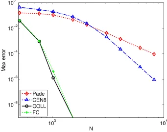
semidiscrete problem is integrated in time using the AB-4 ODE solver for a sufficiently small time-step that the error for the spatial discretization dominates the solution error. (The value ∆t= ∆x/200 was used in all cases.) The resulting system was evolved up to the final time T = 480, just before the solution reaches the right boundary—thus highlighting the character of the FC method as it propagates waves within the interior of the computational domain. (The boundary behavior of the FC method was demonstrated in previous sections.) Figure 3.8 shows that, in this case, the convergence of the FC algorithm closely matches that of Fourier collocation. It should be noted that this example does not capture the error due to the polynomial approximation in the matching regions—this aspect, for which the FC method also displays superior properties, will be considered in detail in Chapter 4.

103 104

10−8 10−6 10−4 10−2 100

N

Max error

[image:45.612.152.493.287.556.2]

Pade CEN8 COLL FC

Figure 3.8: Convergence of the solution of the advection problem (3.3) resulting from use of the eighth-order centered difference, fourth-order Pade-like implicit system, Fourier col-location, and FC differentiation operators.

To examine the performance, demonstrated in Figure 3.8, of the various high-order methods under consideration, Fourier analysis was applied to the semidiscrete problem

(46)

Putting aside at first the particular choice of spatial differentiation approximationD(either that arising from the FC method, or from the other high-order methods considered in Figure 3.8 or, indeed, from any spatial discretization method), a discrete initial condition f(x) may be represented as a linear combination of the Fourier basis functions

ψk(x) =e2πikx/L (3.12)

of the form

f(x) = N/2

X

k=−N/2

fkψk(x) (3.13)

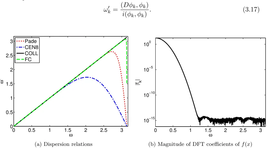
wherefk denote the Fourier coefficients. It is natural and convenient to examine the behav-ior of each basis function independently, since this choice of basis diagonalizes any differ-entiation operator with a translationally invariant kernel [73], such as the finite difference or Fourier collocation schemes. Assuming initial conditionsψk(x), the exact solution of the continuous problem is given ψk(x−t) =ψk(x)ψk(−t).

In the corresponding semidiscrete problem the continuous spatial derivative _∂x∂ is re-placed by the discrete approximation D. Introducing the scaled coordinateyj =N xj/L= xj/∆x and scaled wave-number ωk = 2πk/N (so that ωk ∈ [−π, π] independently of the discretization used), there holds

Dφk(yj) =iωk0φk(yj) (3.14)

where

φk(y) =eiωky, (3.15)

and where ω_k0 is the modified numerical wave-number of the operator. The function ω0 = ω0(ω) for a given discrete operator is called the “dispersion relation” of the operator. The time-dependent factor for the corresponding semidiscrete solutions is given by

φ0_k(−t) =e−iω0kt/∆x. (3.16)

(47)

does not hold exactly, and the dispersion relation may instead be redefined, following [1], by the expression

ω0_k= (Dφk, φk) i(φk, φk)

. (3.17)

0 0.5 1 1.5 2 2.5 3

0 0.5 1 1.5 2 2.5 3 ω ω ’ Pade CEN8 COLL FC

(a) Dispersion relations

0 0.5 1 1.5 2 2.5 3

10−15 10−10 10−5 100 ω |f k |

[image:47.612.116.555.106.348.2]

(b) Magnitude of DFT coefficients off(x)

Figure 3.9: Dispersion relation for various schemes, and decay of the Fourier coefficients of the Gaussian-bump initial condition f(x) =e−(x−10)2

Historically, the dispersion error has been related to the departure of ω0 from ω, that is, by the deviation of the graph ω0 =ω0(ω) from the ideal line ω0 = ω. In Figure 3.9(a) the dispersion relations for the spatial differentiation operators under consideration are compared, and, for reference, in Figure 3.9(b) the Fourier coefficients forN = 5000 points are shown. It can be seen that the coefficients of f(x) vanish to machine precision for all ω ≥ 1.25, restricting the solution to a range of frequencies seemingly well approximated by all of the spatial operators under consideration. Consideration of Figure 3.8, however, shows this not to be the case.

To fully explain this disagreement, closer inspection of the dispersion relation is required. To do this it can be noted that, for each basis function ψk, the error in the approximate solution is given by

|ψk(x)ψk(−t/∆x)−ψk(x)ψk0(−t/∆x)| = |ψk(−t/∆x)−ψ0k(−t/∆x)|

= |e−itωk₋_e−iω0kt/∆x|

(48)

In other words, the approximate solution contains a phase error equal to

t ∆x|ω

0

k−ωk|, (3.19)

large values of which imply that the overall solution is necessarily highly inaccurate. For the example under consideration it is givent/∆x= 480/0.1 = 4800, and hence large errors in the numerical solution may arise even when|ω_k0−ωk|is small. In Figure 3.10, the error estimate 4800|ω_k0 −ωk| is displayed for the various methods under consideration, yielding, in each case, the expected error in the final solution on a per-frequency basis. The results displayed in this figure justify the superior performance of the FC method first observed in Figure 3.8, in spite of the fact that, as noted earlier from consideration of Figure 3.9(a), the dispersion relations for all four differentiation methods under consideration are indistinguishable for values of ω≤1.25, for which the exact solution has Fourier coefficients above the machine precision level.

0

0.5

1

1.5

2

2.5

3

10

−15

10

−10

10

−5

10

0

10

5

ω

4800

⋅

|

ω

’ −

ω

|

[image:48.612.151.494.358.628.2]

Pade

CEN8

COLL

FC

(49)

Chapter 4

Segmentation and parallel

computation

This chapter describes modifications of the basic FC algorithms presented in Chapter 2 that enable implementation of the corresponding FC-based PDE solversfor arbitrary spa-tial dimensions(see Chapters 3 and 5) in cutting edge high-performance parallel computing infrastructures. As shown in this and subsequent chapters, the resulting algorithm is well adapted for execution in specialized modern many-core processors such as GPUs and multi-core CPU clusters, with high-quality parallel scalability and minimal impact on the excellent numerical properties of the underlying numerical methods.

4.1 Thread multiplexing

In some cases it is desirable to configure a parallel computation in such a way that a com-putational task is divided over a large number of threads—possibly in a number of threads that outnumbers the number of available computing cores. In the latter case some or all processors must execute more than one thread, thus giving rise to “thread multiplexing”. Use of thread multiplexing with numbers of threads that far outnumber the numbers of processors can lead to highly efficient load balancing during runtime provided special soft-ware or hardsoft-ware support is available to lessen the overhead associated with switching between threads. In fact, in the GPU literature, the nomenclature “thread-multiplexing” is almost exclusively reserved for such “many-thread-per-core” situations—which, in fact, are particularly well suited for execution in GPU infrastructures.

(50)

languages, including the CUDA programming environment for GPUs as well as the CPU languages Erlang [6], Scala [60], and Go [34]. Not only does multiplexing readily enable dynamic load-balancing, but, for CUDA applications, it is in fact necessary, as discussed below, in order to produce memory-efficient code.

Each SMP on a CUDA-capable device may multiplex over a set of executable threads in order to hide the extremely long latency involved in global GPU memory access. Once a threadblock has made such a memory request, it halts progress until the operation is completed, or “blocks the threadblock”, and the SMP switches to a newready threadblock at a negligible cost. As long as a sufficient number of distinct tasks is available to the SMP, this multiplexing strategy hides the long memory-access times (which in many cases could otherwise dominate the computational cost) by “staggering” many parallel read/writes in time. Effective hiding of memory-access times requires that the problem be subdivided into a number of tasks far outnumbering the number of cores. In addition, the memory footprint of each task must be small enough that many threads can be resident simultaneously within the local memory of an SMP, in order to allow for efficient context switching from blocking to ready threadblocks.

4.2 Line segmentation

The largest atomic unit of computation associated with the FC methodology presented in Section 2.2 is the FFT (direct and inverse) along each line in the domain. While it is possible to implement these transforms in parallel, the communication cost incurred in doing so typically dominates the computational time. Thus parallel FFTs present a significant problem: as larger and larger domains are considered, either the requisite communication (if each FFT is parallelized) or the atomic subcomputations themselves (if separate FFTs are evaluated in separate cores) grow in size without bound. Fortunately the size of the FFTs required by the FC method grows sublinearly, asN1/d, with the overall numberN of unknowns, for a given problem in d-dimensional space. But, if left unchecked, this growth still hinders the GPU performance—as the per-thread memory footprint increases to a level for which a very small number of threads can remain resident per core, and efficient thread multiplexing becomes impossible.

(51)

[image:51.612.186.467.255.431.2]

only requires O(1) storage and computational work per atomic task. In fact, as a by-product of this modification, the overall computational cost required by the FC algorithm is reduced to O(N)—eliminating the logarithmic component arising from the FFT. The modified approach is, in fact, straightforward: the FC method need not be applied to an entire line of points at once. Each line may instead be split into smaller segments consisting of a number ns of discretization points each. The more compact FC operator, now of size ns, is applied independently to each segment.

Figure 4.1: A line containing N = 20 points, split into three segments with ns = 8 points each. Here there are din = 2 points per overlap region (colored in blue), resulting in 7, 6, and 7 interior points for the three segments, from left to right.

(52)

the computation on the segment extending to the left, and another from the segment ex-tending to the right). This ambiguity is resolved by selecting the result from the segment for which the evaluation point is most-internal. If there are an odd number of points in the overlap, the rightmost value is assumed for the (equallydistant) central point.

Remark 4.2.1. The segmentation method described above in this section is a direct gener-alization of the one-dimensional FC solver for periodic problems presented in Section 3.1.1.

A useful feature in this context is that, for interior overlaps where the matching polyno-mials of the FC(Gram) method are not applied at physical boundaries, Gram polynomials of very high degree can be used while retaining stability. In line with the observations made in [1], the value din = 12 provides very high order of accuracy on the interior while still allowing for a stable overall numerical scheme.

For simplicity, convenience and efficiency in GPU implementation, the segmentation structure is constructed in such a way that all the segments have the same size. When a line does not evenly divide into segments of length ns, as is frequently the case, this constraint may be accommodated by simply increasing some of the intermediate segment overlaps. Furthermore, the GPU implementation takes advantage of this structure by re-placing the FFT-based sequence of operations in the FC(Gram) algorithm with a single, dense matrix-vector product (see Remark 4.2.2 below). Matrices corresponding to each type of FC(Gram) operator (differentiation, filtering) are precomputed with respect to the pre-scribed segment sizens. The requirement that segments have a fixed size, which introduces only a small amount of redundant computation, eliminates special cases in the evaluation of the differential operators, and it further improves parallelism in the GPU implementation by guaranteeing thatall of the resulting matrix-vector products have identical dimensions. Note that the order of accuracy of the spatial operator is unaffected—using the same number of matching points d= 5 at all physical boundaries, the only additional approxi-mation introduced by segmentation of the domain is accurate to twelfth order.

(53)

availability of high-performance, small-sized FFT implementations. Special care must be taken in constructing the matrix form, however, or else some numerical precision is lost. In particular, subtractive cancellation effects may be avoided by precomputing the matrix using higher-precision arithmetic—an inexpensive initialization step requiring only O(n2_s) operations.

4.2.1 Stability

When computed via a segmented application of FC(Gram), the filtering operator Sσ is no longer defined continuously over the entire domain. It therefore becomes necessary to consider the action of the operatorSσ on thedinpoints shared by two neighboring segments. Even though this filter serves to dampen higher-frequency oscillations, the Fourier series expansions are necessarily different between the two segments, and therefore the filtered unknown uσ inside of the overlap may disagree when computed from the right or from the left. Since half of the point values of the solution in the overlap are computed from respective Fourier series in the two adjoining segments, the filtering procedure typically introduces a discontinuity within each segment of a size comparable with the numerical error of the solution. In light of the comparatively mild filter used in the FC solvers considered in this thesis, see Chapter 3, this discontinuity is very small, and the methods resulting from the segmented FC method retain numerical stability. For the filter parameter valueα =−ln 10−16 used in [1], on the other hand, a larger mismatch caused by the filter between solutions in neighboring segments occurs and, as has been observed with the solvers presented in this work, the method can become unstable. Thus, the mild filter parameters α=−8µln 10−2 are used for all of the numerical results presented in this thesis.

4.2.2 Dispersion

(54)

0 0.5 1 1.5 2 2.5 3 0

0.5 1 1.5 2 2.5 3

ω

’

Pade CEN8 COLL FC FC, n

s=16

FC, n

s=32

FC, n

[image:54.612.157.493.73.346.2]

s=128

Figure 4.2: Expanded plot of dispersion relations, now including the behavior of segmented FC, for ns equal to 16, 32, and 128. A cursory visual inspection suggests that the rela-tion for ns = 32 is comparable to that of the Pade scheme. In fact, the convergence of the corresponding FC solution is significantly faster than that of the corresponding Pade solution.

corresponding to values of ns equal to 16, 32, and 128. Figure 4.2 shows an expanded set of numerical dispersion relations (comparable to Figure 3.9) which include results for the segmented FC variants. A cursory inspection might suggest that the ns = 32 scheme possesses dispersion characteristics similar to those associated with the spectral-like Pade scheme [48], and that the ns = 16 segmented scheme is significantly more dispersive. As it happens, however, the graphical deviations from the exact line ω0 =ω are insufficient to fully judge the dispersions produced by the algorithm over long distances (cf. Section 3.2.3 for a comparable discussion concerning the unsegmented algorithm). A discussion of the true dispersion character of the segmented FC algorithm is presented in what follows.

GPU Accelerated Fourier Continuation Solvers and Physically Exact Computational Boundary Conditions for Wave Scattering Problems

physically exact computational boundary conditions

for wave scattering problems

Acknowledgements

Abstract

Contents

Part I

Chapter 1

Introduction

1.1

Time domain methods and applications

1.2

Parallel computing

Chapter 2

Fourier continuation

2.1

Fourier continuation based on singular value

decomposi-tion

2.2

Accelerated Fourier continuation based on Gram