Wavelet bispectral analysis for the study of interactions among oscillators whose basic
frequencies are significantly time variable
Janez Jamšek,1,2,3Aneta Stefanovska,1,3and Peter V. E. McClintock3
1Group of Nonlinear Dynamics and Synergetics, Faculty of Electrical Engineering, University of Ljubljana, Tržaška 25, 1000 Ljubljana, Slovenia
2
Department of Physics and Technical Studies, Faculty of Education, University of Ljubljana, Kardeljeva ploščad 16, 1000 Ljubljana, Slovenia
3
Department of Physics, University of Lancaster, Lancaster LA1 4YB, United Kingdom 共Received 24 April 2007; published 24 October 2007兲
Bispectral analysis, recently introduced as a technique for revealing time-phase relationships, is extended to make use of wavelets rather than Fourier analysis. It is thus able to encompass instantaneous phase-time dependence for the case of two or more coupled nonlinear oscillators. The method is demonstrated and evaluated by use of test signals from a pair of coupled Poincaré oscillators. It promises to be useful in a wide range of scientific contexts for studies of interacting oscillators whose basic frequencies are significantly time variable.
DOI:10.1103/PhysRevE.76.046221 PACS number共s兲: 05.45.Xt, 05.45.Tp, 02.70.Hm
I. INTRODUCTION
Coupled oscillatory systems are found in a diversity of different contexts in science and technology, including, e.g., engineering structures such as bridges关1,2兴, the flashing of male fireflies 关3兴, the mammalian cardiorespiratory system 关4,5兴, the physics of plasmas关6兴, laser arrays关7兴, and chaos 关8兴. Their understanding requires a knowledge of the int-eroscillator interactions, and a common problem lies in ex-tracting this information from measurements of oscillator co-ordinates, usually recorded in the form of time series. Where bivariate data are available for a pair of interacting oscilla-tors共i.e., where the coordinate of each of them can be mea-sured separately兲, phase relationships can be obtained by use of the methods recently developed for analysis of synchroni-zation, or generalized synchronisynchroni-zation, between chaotic and/or noisy systems. Not only can the interactions be de-tected关9兴, but their strength and direction can also be deter-mined关10兴. The next logical step in studying the interoscil-lator interactions from measured data was to determine the type of the couplings 关11兴, as the methods developed for synchronization analysis are not capable of answering this question.
Systems are usually taken to be stationary. In reality, how-ever, mutual interactions among their subsystems often result in time variability of the characteristic frequencies. Fre-quency and phase couplings sometimes occur only tran-siently, and the strength of coupling between pairs of indi-vidual oscillators may change with time. Under these circumstances, conventional bispectral analysis for stationary signals, based on time averages, is no longer sufficient. Rather, the time evolution of the bispectral estimates is needed. Priestley and Gabr 关12兴 were probably the first to introduce the time-dependent bispectrum for harmonic oscil-lators. Most subsequent work has been related to the time-frequency representation and is based on high-order cumu-lants关13兴. An extensive overview can be found in关14兴.
Schacket al.关15兴have recently introduced a time-varying spectral method for estimating the bispectrum and
bicoher-ence: they obtain estimates by filtering in the frequency do-main and then obtaining a complex time-frequency signal by inverse Fourier transform. They assume, however, that the interacting oscillators are harmonic. Millingenet al.关16兴 in-troduced the wavelet bicoherence and were the first to dem-onstrate the use of bispectra for studying interactions among nonlinear oscillators. They used the method to detect peri-odic and chaotic interactions between two coupled van der Pol oscillators, but without concentrating on time-phase re-lationships in particular.
In an earlier paper关11兴, we extended bispectral analysis to encompass time dependence, and demonstrated the potential of the enhanced technique to determine the types of coupling among interacting nonlinear oscillators. Time-phase cou-plings can be observed by calculating the bispectrum and adapted bispectrum, thereby obtaining the time-dependent biphase and biamplitude. This method has the advantage that it allows an arbitrary number of interacting oscillatory pro-cesses to be studied. It is applicable both to univariate 共a single signal from the coupled system兲, and to multivariate data共a separate signal from each oscillator兲. It yields results that are applicable quite generally to any system of coupled nonlinear oscillators.
In the present paper, we introduce a new technique likely to be useful for studying complex oscillatory systems whose characteristic frequencies vary in time, e.g., the human car-diovascular system关5兴. It is able to reveal both the existence of interactions among the subsystems, and also the nature of the interactions. Cardiovascular signals are highly complex from the nonlinear dynamics point of view. Their frequencies and amplitudes, and the couplings among the subsystems, are all time variable. To be able to cope with this type of signal we have incorporated wavelets into the technique and further extended it for studying the instantaneous phase cou-plings.
cardiovas-cular system itself, currently in progress, will be described elsewhere.
In Sec. II we introduce the technique and in Sec. III we describe how it has been tested on a model coupled-oscillator system. The relative advantages and disadvantages of the Fourier and wavelet bispectral methods are discussed in Sec. IV. Finally, in Sec. V we summarize the results obtained and draw conclusions.
II. METHOD
A. Time-phase bispectral analysis
We start by summarizing briefly the salient features of time-phase bispectral analysis as based on the Fourier trans-form. For a detailed discussion, see关11兴.
The classical bispectrum estimate is obtained as an aver-age of estimated third-order moments 共cumulants兲 Mˆ3i共k,l兲 关17兴,
Bˆ共k,l兲= 1 K
兺
i=1K
Mˆ3i共k,l兲, 共1兲
where the third-order moment estimateMˆ3i共k,l兲is performed by a triple product of discrete Fourier transforms共DFTs兲at discrete frequenciesk,l, and k+l,
Mˆ3i共k,l兲=Xi共k兲Xi共l兲Xiⴱ共k+l兲. 共2兲 Herei= 1 , . . . ,Klabel the time segments into which the sig-nal has been divided. The bispectrum B共k,l兲 is a complex quantity, defined by magnitudeAand phase,
B共k,l兲=兩B共k,l兲兩ej⬔B共k,l兲=Aej. 共3兲 For each共k,l兲, the value of B共k,l兲 can be represented as a point in the space, Re关B共k,l兲兴versus Im关B共k,l兲兴, thus defin-ing a vector whose magnitude共length兲is known as the bi-amplitude. The phase is determined by the angle between this vector and the positive real axis and for the bispectrum is called the biphase.
To encompass time dependence within bispectral analysis in analogy with the short-time Fourier transform, we can move a time windoww共n兲of lengthMacross the signalx共n兲 and calculate the discrete Fourier transform at each window position,
X共n,k兲 ⬵ 1 M
兺
i=0M−1
x共i兲w共i−n兲e−j2ik/M, 共4兲
wherekis the discrete frequency andnthe discrete time. The instantaneous biphase calculated from Eqs. 共1兲 and 共3兲 is then
共k,l,n兲=k共n兲+l共n兲−k+l共n兲. 共5兲 Simultaneously, we observe the instantaneous biamplitude, from which it is possible to infer the relative strength of the interaction. It is thus possible to detect and quantify the pres-ence of coupling among the oscillators and to follow its per-sistence in time.
B. Wavelet bispectrum
The Fourier transform is based on the presumptions of共a兲 periodicity and共b兲infinite length of the signal series关18,19兴. Because neither assumption can be strictly true for any mea-sured signal, the determination of separate frequencies in a system that possesses strong couplings is very demanding. The difficulty is greater in the low-frequency range, which is of particular interest to us, because the characteristic fre-quencies are close to each other and are therefore even harder to separate. The uncertainty principle governing the Fourier transform limits its ability to separate harmonic com-ponents in the frequency domain of the bispectrum关20,21兴. This might cause problems for detection of quadratic phase couplings in the case of frequency pairs that are close to-gether. To ensure good resolution of low frequencies, we need longer sections for calculation of the discrete Fourier transform. This immediately decreases the number of sec-tions possible and weakens the bispectrum estimation. How-ever, we cannot use longer signals, because they lead to non-stationarity, and the variance consequently becomes even larger 关22兴. One way of accommodating these conflicting demands is through the introduction of wavelet analysis.
Wavelet analysis can be seen as a generalization of Fou-rier analysis 关21兴 by the addition of time resolution—in a more fundamental way than is permitted by the short-time Fourier transform 共STFT兲 关23兴. Wavelet analysis has been applied with considerable success to cardiovascular data 关24兴. A generalization of bispectral analysis, based on wave-lets, may be expected to be able to detect temporal variations in phase coupling, or short-lived couplings, and to cope with broadened and coalescing peaks that cannot be resolved due to the time-frequency resolution restrictions that govern the STFT-based bispectrum.
Wavelet analysis was first introduced by Morlet 关25兴. It enables the window length to be adjusted to the frequency currently being analyzed. It is a scale-independent method. It uses a window function known as the mother wavelet, or basic wavelet共u兲, which can be any function that satisfies the wavelet admissibility condition关21兴. This function intro-duces a scales共its width兲into the analyses. Commitment to any particular scale is avoided by using all possible scalings of共u兲. The mother wavelet is also translated along the sig-nal to achieve time localization. Thus, a family of generally nonorthogonal basis functions is obtained,
⌿共s,t兲=兩s兩−p
冉
u−ts
冊
. 共6兲 The parameter p is an arbitrary non-negative number, used for normalization. Values of p of 0, 1/2, and 1 are encoun-tered in the literature关26兴. The prevailing choice of p= 1 / 2 yields a factor兩s兩−1/2and ensures energy conservation. In this case, the L2 norm of the wavelet, and thus its energy, is unaffected by the scaling operators. The continuous wavelet transformWg共s,t兲of a signalg共t兲 is defined as:Wg共s,t兲=
冕
−⬁⬁
⌿ⴱ
冉
−ts
冊
g共兲d 共7兲In numerical applications, the scales and time t are re-stricted to take discrete values. A natural discretization of the scaling parameter issm=m, wherem僆Z, and the step is a positive number⫽0 , 1. Within the scalem, the signal is sampled only at timestn=nm, which means that the sam-pling rate is automatically adjusted to the scale关21兴.
For different values of m and n, we obtain the discrete wavelet family
⌿m,n共u兲=−m/2共−mu−n兲, 共8兲 where we have setp= 1 / 2. The discrete wavelet transform, defined by this family, is simply a sampled version of Wg共s,t兲. By choosing near 1, we can obtain a representa-tion close to the continuous transform.
1. Direct relationship between the scale and the frequency using Morlet wavelets
Coupling between wavelets makes sense when a fre-quency can be assigned to the wavelet. We restrict our atten-tion to wavelets whose Fourier transforms exhibit a single dominant peak, and we define the location of that peak as being the corresponding frequency. In the literature关21兴, sev-eral suitable wavelets are mentioned. Following earlier en-ergy density studies of measured cardiovascular signals, the Morlet mother wavelet was chosen关24兴.
Morlet proposed the use of a Gaussian function modu-lated by a sine wave. Its Fourier transform is a shifted Gauss-ian, adjusted slightly so that the admissibility condition ˆ共0兲= 0 is satisfied:
ˆ共f兲=
冑
2 1冑
4 共e−42共f−f
0兲2/2−e42f2/2−e42f0 2
/2兲. 共9兲
The corresponding time domain expression is 共u兲=−1/4共e−j2f0u−e42f0
2
/2兲e−u2/2. 共10兲
The choice off0 represents a compromise between localiza-tion in time and in frequency. For smallerf0, the shape of the wavelet favors localization of singular time events whereas, for larger f0, more periods of the sine wave within the win-dow improve the frequency localization. For f0⬎0.8, the value of the second term in共10兲 is so small that it can be ignored in practice, and a simplified expression for the Mor-let waveMor-let in the time domain is
共u兲=−1/4e−j2f0ue−u2/2. 共11兲
The corresponding wavelet family consists of Gaussians cen-tered on a time t and with standard deviations. In the fre-quency domain, we have Gaussians with a central frefre-quency f=f0/sand a standard deviation of 1 / 2冑2s. Thus, applica-tion of the wavelet transform at a given scalescan also be interpreted as bandpass filtering, giving an estimation of the contribution to the frequencies in this band. The relationship between the scale and the central frequency for the Morlet wavelet is then
f= f0
s. 共12兲
The frequency resolution changes with frequency. At low frequencies共large scales兲, the resolution is better than at the high frequencies 共small scales兲. Accordingly, the time reso-lution is better for high-frequency than it is for low-frequency components. In order for peaks to be detected atf1 and f2 共f1⬎f2兲, they must be separated by at least one-half of the standard deviation of the peak at the higher frequency, thus requiringf1−f2ⱖf1/ 4f0. The choice of f0determines the current frequency resolution. By choosing f0= 1, we ob-tain a simple relation between scale and frequency, f= 1 /s. Slow events are examined with a long window, while a shorter window is used for faster events. The Morlet wavelet provides optimal time-frequency localization within the lim-its imposed by the uncertainty principle.
2. Definition of the wavelet bispectrum
For the case of the wavelet bispectrum, the definitions are analogous to those used in Fourier-based bispectral analysis 关16,17兴. The wavelet bispectrum共WB兲BWis given by
BW共s1,s2兲=
冕
TWg共s1,兲Wg共s2,兲Wgⴱ共s,兲d, 共13兲
where
1 s1+
1 s2=
1
s. 共14兲
The WB measures the amount of phase coupling in the in-terval T that occurs between wavelet components of scale lengthss1,s2, ands of a signalg共t兲, in such a way that the frequency sum rule共14兲is satisfied. It is a complex quantity, defined by its magnitudeAand phase:
BW共s1,s2兲=兩BW共s1,s2兲兩ej⬔BW共s1,s2兲=Aej. 共15兲 The instantaneous biphase calculated from共13兲and共15兲is
共s1,s2,t兲=s1共t兲+s2共t兲−s共t兲. 共16兲
If two scale components s1 and s2 are scale and phase coupled, s=s1+s2, it holds that the biphase is 0 共2兲 rad. For our purposes, the phase coupling is less strict because scale-dependent components can be phase delayed. We consider phase coupling to exist if the biphase is constant 共but not necessarily 0 rad兲for at least several periods of the highest scale component.
Simultaneously, we observe the instantaneous biampli-tude, from which it is possible to infer the relative strength of the interaction
A共s1,s2,t兲=兩BW共s1,s2,t兲兩. 共17兲 Analogously to the case of the Fourier cross bispectrum, one can define a wavelet cross bispectrum as
BWcfgg共s1,s2兲=
冕
TWf共s1,兲Wg共s2,兲Wgⴱ共s,兲d. 共18兲
bispectrum 共FB兲 BF 关27兴. The nonredundant region of the WB is called its principal domain. The principal domain can be further divided into two triangular regions in which the WB has different properties关28兴: the inner triangle共IT兲, and the outer one. Our interest centers on the IT关22,29兴.
3. Wavelet bispectrum adapted to real signals
The relationship between the frequency 共scale兲 and the width of the window used for calculation of the wavelet transform is hyperbolic. A log-log scale is therefore a natural choice for its presentation. However, to be able to comply with the frequency共scale兲sum rule共14兲, we need to achieve better frequency共scale兲resolution for high frequencies共low scales兲as can be effected by use of the Morlet wavelet when f0 is chosen to be 1. Otherwise, nearby peaks at high fre-quencies cannot be resolved. For this purpose we introduce parametersd andaminto the Morlet wavelet
共u兲=amcne−2f0ue
−u2/d
, 共19兲
where the constantcn= 3.9487−1/4. The parameter d deter-mines the exponential decay of the Gaussian. This attenuates the Morlet wavelet, and thus permits the choice of a suitable combination of time and frequency 共scale兲 resolution. The time resolution is⌬t=sd, given by the decay of the exponen-tial part of the wavelet. Asdincreases共d⬎1兲, the frequency 共scale兲 resolution improves, whereas the time resolution de-teriorates;d is set such that the Gaussian function decays to 0.001 for each scale. A high value ofd would cause a non-zero value of the Morlet window at its edges, resulting in side lobes on the WB. Ifd were infinite, the Morlet window would become a unit window, and the wavelet transform would become the selective discrete Fourier transform 共SDFT兲 关31兴. We wish to choose the frequencies in the analy-sis procedure freely, i.e., not restricted tos僆兵2n其, which im-plies a certain redundancy in the wavelet transform coeffi-cients.
The frequency resolution at high frequencies is still insuf-ficient: it is necessary to increase the length of the Morlet wavelet for high frequencies. This can be achieved in differ-ent ways. Figure1shows the hyperbolic decay of the Morlet wavelet length with increasing frequency 共solid line兲. The wavelet length can be multiplied by a factoram, equal to that for the lowest frequency of interest, and then increased with increasing frequency,
am= 21.8共f−fmin兲/共fmax−fmin兲, 共20兲 where f= 1 /s is the frequency of observation, and fmin and fmaxdefine the frequency range of interest. The constant, 1.8, is set experimentally. In this way, we obtain the dotted line in Fig.1. As the wavelet length is prolonged for high frequen-cies, the frequency resolution increases, whereas the time resolution deteriorates. Another way to obtain the necessary frequency resolution is to use a fixed wavelet length for all high frequencies, as shown by the dash-dotted line in Fig.1. WB estimation using the Morlet mother wavelet encoun-ters a normalization problem. For each scale, a window of different length is used. In the case of a signal composed of different frequency components, but equal Fourier powers, this would result in different wavelet spectral energies for different frequencies. Two couplings among different fre-quencies with the same Fourier powers and the same nature of coupling, would result in different coupling strengths in the wavelet bispectrum. In共6兲, a factor兩s兩−1/2is used to en-sure energy preservation. We choose to use a factor 1 /NW instead, whereNWis the Morlet window length. In this way, we can compare results obtained using FB and WB, since both preserve energy.
Normalization of the WB is achieved in the same way as for the FB 关11兴. The normalized WB indicates the average level of quadratic nonlinear phase coupling and, in a way, serves as an indicator of how non-Gaussian the signal is关32兴. The critical values for the WB and biamplitude estimates were normalized to 1. If the estimated value is higher than the average value of WB in the IT, then it is taken as valid. By critical value, we mean that a value exceeds the noisy background共other than Gaussian兲, rounding, and estimation errors.
4. Instantaneous frequency
The bispectrum is sensitive to time variations of the fre-quency components, and it acquires a characteristic diagonal elongation of peaks. Bifrequencies where peaks in the bispectrum 共wavelet兲 provide evidence of possible phase and/or frequency interactions are further studied by calcula-tion of the biphase and biamplitude as funccalcula-tions of time. In doing so we do not follow time variations of the frequencies in the bifrequency pair when estimating time-biphase or -biamplitude dependence. They are estimated only for the peak bifrequency, i.e., where the average amplitude in the bispectrum takes its highest value. If the bifrequencies change considerably during the time of observation, such an approach can yield misleading results. It is of course possible to calculate the biphase and biamplitude for all the bifre-quencies near the peak bifrequency and to plot them simul-taneously in a graph, thus obtaining the time variations of the coupled frequency components and the evolution of the bi-phase and biamplitude. The interpretation, however, is rather difficult.
To be able to trace changes in the bifrequency 共f1,f2兲 under study, we need to incorporate the instantaneous fre-quencies 关33兴 f1共t兲 and f2共t兲 into the bispectral analysis. In this way we can calculate the instantaneous biphase and in-stantaneous biamplitude for the inin-stantaneous bifrequency 0 0.2 0.4 0.6 0.8 1 1.2 1.4 2
0 20 120
f (Hz)
N W
(s)
FIG. 1. Variation of the lengthsNWof Morlet-like wavelets with
frequency 共scale兲: Morlet wavelet 共solid line兲; adapted Morlet wavelet共dotted line兲; and fixed wavelet length for high frequencies
[image:4.612.95.251.60.130.2](f1共t兲,f2共t兲). Such an approach should lead to better results for the time dependence of the biphase and biamplitude. There are two main methods to determine the instantaneous frequency of an oscillatory process, based on 共i兲 marked events, and共ii兲an analytic signal.
The marked events method involves marking events that indicate completion of one cycle of oscillation. The frequen-cies determined from sequential pairs of marked events are then linearly interpolated to obtain instantaneous values. Minimal or maximal values of the signal are usually taken as marked events. For instance, the R peak is strongly pro-nounced in an electroencephalogram共ECG兲signal. It is eas-ily distinguishable and can be automatically detected. The marked events approach can be applied easily in the case of signals where one oscillatory component dominates. How-ever, not all processes in the blood distribution system can be measured selectively. Most of the quantities that can be mea-sured, such as cardiovascular signals 关24兴, contain multiple oscillatory processes and maxima and minima are no longer uniquely determined.
The second approach is based on the Hilbert transform 关34兴. From the signal under observation, x共t兲, we construct an analytic signal
共t兲=x共t兲+ixH共t兲=A共t兲ej共t兲, 共21兲
which is a complex function of time. The functionxH共t兲 is the Hilbert transform ofx共t兲:A共t兲and共t兲are, respectively, the instantaneous amplitude and phase. The instantaneous frequency f共t兲 can be obtained by numerical differentiation of共t兲. In general, this may result in very large fluctuations in the estimate off共t兲due to the influence of noise and/or the complicated form of the signal. Although共t兲can be calcu-lated formally for arbitraryx共t兲, it has a clear physical mean-ing ifx共t兲is a narrowband signal, in which case the instan-taneous frequency corresponds to that of the maximum in the instantaneous spectrum. Several methods are available for estimation of f共t兲in the共usual兲case where we are not inter-ested in the behavior of a frequency on time scales smaller than its characteristic oscillation period关35兴.
We suggest a combination of both methods to obtain the instantaneous frequencies of oscillatory processes in the car-diovascular system, depending on the shape of the signal under scrutiny. The instantaneous frequency of cardiac oscil-lations is best calculated from ECG and blood pressure sig-nals using the marked events method. Marked events can also be used to obtain the instantaneous frequency of the respiratory oscillations directly from the respiration signal, whereas the analytic signal procedure is best applied to cal-culate the instantaneous respiratory frequency from blood flow signals. In the latter case the signal must first be band-pass filtered in the frequency domain, by assigning zero val-ues to all amplitudes outside the respiratory frequency range 关30兴.
Note that the phase can also be obtained by direct use of the coefficients of the complex continuous wavelet transform 关36兴, a method that has been shown to yield a precision com-parable to that obtained by the marked events method and the Hilbert transform. The combination of the wavelet
trans-form and the bispectral analysis may further improve the precision of phase detection, as the phases obtained are con-tinuous and the trade-off between frequency and time local-ization may further be optimized by taking account of the second-order statistics of the bispectra. However, this is a matter that needs additional investigation and will be re-ported elsewhere in due course.
III. ANALYSIS
A. Test signal
To illustrate the essence of the method, and to test it, we use a generic model of two interacting systems whose basic unit is the Poincaré oscillator
x˙1= −x1q1−1y1+2共x1−x2兲2+共t兲,
y˙1= −y1q1+1x1+2共y1−y2兲2,
x˙2= −x2q2−2y2,
y˙2= −y2q2+2x2,
qi=␣i共
冑
xi2+yi2−ai兲. 共22兲 The activity of each subsystem is described by the two state variablesxiandyi, wherei= 1 , 2 denotes the subsystem, ␣i, ai and i are constants, and 2 is the coupling amplitude. The parameters of the model are set to ␣1= 1,a1= 0.5, and ␣2,a2= 1. Here 共t兲 is zero-mean white Gaussian noise 具共t兲典= 0,具共t兲,共0兲典=D␦共t兲, andD= 0.08 is the noise inten-sity.The test signal is the variablex1A共t兲of the first oscillator, recorded as a continuous time series as shown in Fig.2共a兲. Prior to analysis, the signal was first normalized between 0 and 1 and its mean value was subtracted. For the first 400 s, there was quadratic coupling with 2= 0.2. After a further 400 s, the forcing was removed by setting2= 0. During the last 400 s, the coupling was increased again to2= 0.2. In the latter case the characteristic frequency of the second oscilla-tor was both modulated and linearly increased from f2 = 0.25 to 0.35 Hz, as shown in Fig. 3共a兲. The first 15 s of each of the three coupling modes are shown in Fig.2共a兲, with the corresponding power spectra in Fig.2共b兲.
A standard fourth-order Runge-Kutta method共RK4兲 was used for the numerical integration. The initial values and step size were set to x1= −0.1, y1= 1.0, x2= −0.1, y2= 1.0, h = 0.01. The signalx1 was than resampled to 10 Hz.
B. Wavelet bispectrum
coupling. The test signal x1A clearly has richer harmonic structure in the presence of nonlinear coupling. In addition to the characteristic frequency of the first oscillator, it contains components with frequencies 2f1, 2f2,f1+f2, and f1−f2. As well as having a particular harmonic structure, the compo-nents of the signal x1A also have related phases 21, 22, 1+2, and 1−2.
For bispectral analysis the whole signal is analyzed as a single entity, after the transients caused by the changes in coupling strength have been removed. First the WB is esti-mated, as shown in Figs. 4共a兲 and 4共b兲. Close inspection shows that all the peaks expected to arise from bispectral analysis of the nonlinear interaction between the two oscil-lators f1 and f2 are indeed present. Quadratic coupling has already been discussed in detail in关11兴and is not a subject of this paper.
Bifrequencies where peaks provide evidence of possible frequency interactions are then further studied by calculation of the biphase and biamplitude as functions of time. Diago-nal elongation of peaks in the bispectrum demonstrates time variation of the corresponding frequency components. The characteristic frequency of the second oscillator f2 varies
within 0.25–0.35 Hz. Our primary interest lies in the bifre-quency共f1,f2兲. The time evolution of its biphase and biam-plitude are shown in Figs. 4共c兲 and 4共d兲. The results for nonzero coupling are quite different from those where cou-pling is absent共the second 400 s兲. The biphase is constant in the presence of quadratic coupling共first 400 s兲 and the bi-amplitude is above zero. Let us concentrate on the third 400 s, where one of the bifrequency components is varying. In the bispectrum we concentrate on the peaks where possible phase and/or frequency couplings are occurring. Here, we estimate the time evolution of the biphase for the peak bifre-quency, i.e., where the average biamplitude takes its highest value. This is why, near 800 s where the characteristic fre-quency of the second oscillator f2 has not risen much above 0.25 Hz, we obtain constant biphase and high biamplitude as shown in Figs. 4共c兲 and4共d兲. As f2 continues to grow lin-early 共but with modulation兲 to 0.35 Hz, the biamplitude drops toward zero and the biphase exhibits phase slips, falsely suggesting that there is no coupling.
C. Instantaneous frequency
Figures5共a兲and5共b兲show the biphase and biamplitude, taking explicit account of the instantaneous bifrequency. In
0 15 0 15 0 15
−0.5 0.5
(a)
x1A
(t)
(arb.
units)
Time (s)
0 2.5 0 2.5 0 2.5
0 1
(b)
P(x
1A
)
(arb.
units)
f (Hz)
f1−f2 f1 f1+f2
f2 f1 f1
f2 f1+f2
f1−f2
[image:6.612.345.528.55.326.2](1) (2) (3)
FIG. 2. Simulation results for a pair of quadratically coupled Poincaré oscillators in the presence of additive Gaussian noise.共a兲 The test signalx1A共t兲 from the first oscillator, after normalization
and subtraction of its mean value. The first oscillator has a charac-teristic frequency f1= 1.1 Hz. That of the second oscillator is f2
= 0.25 Hz. The oscillators are unidirectionally and quadratically coupled with three different coupling strengths: in column共1兲 2
= 0.2,共2兲0, and共3兲0.2. In column共3兲the characteristic frequency of the second oscillator is linearly increased fromf2= 0.25 to 0.35 while being at the same time modulated with 0.0013 sin共20.01t兲. Each coupling lasts for 400 s. The sampling frequencyfs= 10 Hz. Only the first 15 s are shown in each case.共b兲The corresponding power spectra ofx1A共t兲.
(a)
(b)
0 400 800 1200
0.9 1
f 1
(Hz)
Time (s)
0 400 800 1200
0.25 0.37
f 2
(Hz)
[image:6.612.94.252.60.177.2]Time (s)
FIG. 3. Instantaneous frequencies of共a兲the first oscillatorf1and
共b兲the second oscillatorf2, used for generating the test signalx1A.
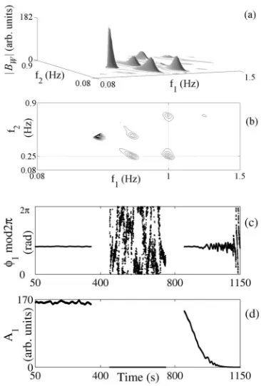
FIG. 4. 共a兲The modulus of the wavelet bispectrum兩BW兩 calcu-lated for K= 34 segments, 67% overlapping, with Tm= 8 s, Ge
= 0.001, using a fixed Morlet wavelet length ofTHF= 40 s for
cal-culation of the high frequencies. 共b兲 A contour plot of the WB. Abovef2⬎0.9 Hz, the wavelet bispectrum is removed because the
triplet共1.1 Hz, 1.1 Hz, 1.1 Hz兲 produces a high peak that is not physically significant.共c兲 The biphase1 and共d兲 the biamplitude A1for the bifrequency共1 Hz, 0.25 Hz兲peak 1, calculated using a
[image:6.612.83.264.617.705.2]doing so, the instantaneous frequencies f1共t兲and f2共t兲 关Figs.
3共a兲and 3共b兲兴were both obtained using the marked events method. The results for nonzero coupling are quite different from those where coupling is absent 共second 400 s兲. The biphase is constant in the presence of quadratic coupling 共first 400 s兲and the biamplitude takes a finite value. During the final 400 s, when there is a large time-frequency variation of the second oscillator’s frequency, the biamplitude is again above zero and the biphase remains constant during the whole time of observation—both features being clearly re-solved despite the nonlinear coupling. Bispectral analysis was also performed using instantaneous frequenciesf1共t兲and f2共t兲, where both of them were obtained directly from Eq. 共22兲. The results were exactly the same.
IV. COMPARISON OF FOURIER- AND WAVELET-BASED BISPECTRA
We now present some simulation results to illustrate the main reason for sometimes preferring to use wavelet-based rather than Fourier-based bispectra. We then discuss the main strengths and weaknesses of the two methods.
We again use the same generic model, Eq.共22兲with qua-dratic coupling, now taking f1= 1.1 Hz and f2= 0.24 Hz. The model parameters␣i,ai, andDare the same as for the test signal x1A 关Fig. 2共a兲兴. In this way, we obtain the test signalx1B共t兲 shown in Fig. 6共a兲from the first oscillator, re-corded as a continuous time series. The two coupling strengths of 2= 0 共no coupling兲 and 2= 0.2 共weak cou-pling兲 are interchanging every 20 s. Only the first 15 s of x1B共t兲are shown for each coupling mode. The corresponding power spectra are shown on Fig.6共b兲.
Figures 7共a兲 and 7共b兲 show the FB in perspective and contour plots, respectively, for the test signalx1B. We con-centrate on the bifrequency of primary interest,f1共t兲,f2共t兲. In the first case a 100 s window was used for estimating DFTs. Details of how to choose the window length are given in 关37兴. The calculated instantaneous biamplitude and biphase
are presented in Figs.7共c兲 and 7共d兲. The biphase increases monotonically and there are no episodes of constant biphase, although the biamplitude remains high during the whole time of observation.
In a second set of calculations, a 130 s window was used for estimating DFTs. The corresponding biamplitude and bi-phase are shown in Figs.7共e兲and7共f兲. The biphase tends to be constant共remains within a / 2 range兲 and the biampli-tude is high 共more than twice the average value of the FB within the inner triangle兲.
It is evident that, for the detection of short episodes共⬍12 the DFT window length兲 of nonlinear coupling, the FT method is not appropriate. It can lead to misleading interpre-tation of the bispectral estimates, either of no coupling in the first case or of quadratic coupling in the second case.
Figures 8共a兲 and 8共b兲 show the WB in perspective and contour views, respectively, for the same signal x1B. The wavelet-based method clearly gives the same information about the peak’s relative amplitude and bifrequency as the Fourier-based method, but the frequency resolution is evi-dently lower than in the latter case. The calculated instanta-neous biamplitude and biphase are presented in Figs. 8共c兲
and8共d兲respectively. They clearly reveal the intervals dur-ing which the coupldur-ing is present or absent. By increasdur-ing the time resolution for calculation of the WB at high frequen-cies, we obtain precisely the times at which the intermittent quadratic coupling occurs, i.e., every 20 s, Fig.8共e兲and8共f兲.
A. Overview of main advantages and weaknesses of Fourier and wavelet bispectra
We now overview the relative strengths and weaknesses of the Fourier-based and wavelet-based methods of calculat-ing bispectra. There are several points to consider.
共1兲 Time and frequency resolution. To observe a given
50 400 800 1150
−7 18
φ 1
(rad)
Time (s)
50 400 800 1150
0 180
A 1
(arb.
units)
[image:7.612.348.526.59.197.2](b) (a)
FIG. 5. Wavelet bispectral estimates based on the instantaneous frequenciesf1共t兲 and f2共t兲, which were obtained using the marked
events method.共a兲The instantaneous biphase1and共b兲the instan-taneous biamplitudeA1for the bifrequency共1.1 Hz, 0.25 Hz兲peak
1, calculated forK= 34 segments, 67% overlapping, withTm= 8 s,
Ge= 0.001, using a fixed Morlet wavelet length ofTHF= 40 s for the
calculation of high frequencies and a 0.1 s time step.
0 15 0 15
−1.3 1.3
(b)
x 1B
(t)
(arb.
units)
0 2.5 0 2.5
0 1
P(x
1B
)
(arb.
units)
f (Hz)
(a)
Time (s)
(1) (2)
f1
f2 f1+f2
f1−f2
f1
FIG. 6. Simulation results for time-intermittent quadratic cou-plings in the presence of additive Gaussian noise.共a兲The test signal
x1B共t兲 from the first oscillator, with characteristic frequency f1
= 1.1 Hz. The characteristic frequency of the second oscillator was
f2= 0.24 Hz. The oscillators are unidirectionally and quadratically
coupled with two different coupling strengths: column共1兲 2= 0; and共2兲 2= 0.2. The coupling in column 共2兲is present every 20 s
and lasts for 20 s. The signal is 1200 s long and sampled with sampling frequency fs= 10 Hz. Only the first 15 s are shown in
[image:7.612.84.264.60.188.2]frequency, the signal must be observed over at least one pe-riod of this frequency, which inevitably limits time localiza-tion. Due to the uncertainty principle关21兴, sharp localization in time and frequency are of course mutually exclusive:
⌬t⌬f= 1
4, 共23兲
wheretis the time interval and f is the frequency band. The equality holds if and only if the window is Gaussian.
In general, the WB detects intermittent phase couplings well, whereas the FB averages out most of the time-relevant information. The triplet共f1,f2,f3兲 results in a high peak in the bispectrum if the coupling condition f3=f1+f2, is satis-fied共within the frequency resolution兲. Because the frequency resolution changes with frequency, this condition is less strict for WB analysis. If there is a mismatch in the coupling fre-quencyfsuch thatf3=f1+f2+⌬f, where⌬fis larger than the frequency resolution of the FB but smaller than the WB fre-quency resolution, then the WB will peak for the triplet 共f1,f2,f3兲, whereas the FB will not. By increasing the
fre-FIG. 7. Analyses of the test signal with time-intermittent qua-dratic couplings, in the presence of additive Gaussian noise using the Fourier-based bispectral method.共a兲The Fourier-based bispec-trum兩BF兩for signalx1Bcalculated withK= 33 segments, 66% over-lapping and using the Blackman window to reduce leakage and共b兲 its contour view. The part of the bispectrum abovef2⬎1.0 Hz has been cut because the triplet共1.1 Hz, 1.1 Hz, 1.1 Hz兲 produces a high peak that is physically meaningless.共c兲 The biphase1. 共d兲
[image:8.612.347.528.55.467.2]The biamplitudeA1for the bifrequency共1.1 Hz, 0.24 Hz兲, calcu-lated with a 100-s-long window for estimating DFTs.共e兲The bi-phase and共f兲the biamplitude calculated with a 130 s window for estimating DFTs. In both cases, a 0.3 s time step was used and the Blackman window was applied.
FIG. 8. Analyses of a test signal for time-intermittent quadratic couplings in the presence of additive Gaussian noise using the wavelet bispectral method.共a兲The wavelet bispectrum兩BW兩 calcu-lated withK= 33 segments and 66% overlapping. The part of the bispectrum above f2⬎1.0 Hz is removed, because the triplet 共1.1
Hz, 1.1 Hz, 1.1 Hz兲produces a high peak that is physically mean-ingless.共c兲The biphaseand共d兲 biamplitudeA1for bifrequency 共1.1 Hz, 0.24 Hz兲, calculated withGe= 0.01.共e兲The biphaseand 共f兲biamplitude A1, calculated with Ge= 0.0001. In both cases, the time step was 0.1 s,Tm= 8 s, and aTHF= 20 s fixed Morlet wavelet
[image:8.612.84.264.57.463.2]quency resolution of the WB 共increasing the length of the Morlet wavelet for high frequencies兲we obtain approximate results, as can also be obtained with the FB.
On the other hand, if there is a brief episode of coupling between the oscillators, the FB-based method cannot detect it from the signal due to the large time window used, whereas the WB will detect it, down to a certain minimum duration. Thus the WB allows intermittent couplings to be detected. When applying the FB to real data, we have to ensure the necessary frequency resolution to be able to distinguish sepa-rate frequency components and at the same time achieve suf-ficient time resolution to be able to detect the onset of cou-plings among the cardiovascular oscillators. The scope for choice of window length is limited by the uncertainty prin-ciple 关21兴, and compromise is inevitably needed between time and frequency resolution.
In contrast to the FB, the WB based on Morlet’s mother wavelet enables us to enjoy optimal time and frequency reso-lution at the same time, which is an obvious advantage com-pared to the FB.
Since the time resolution of the WB is higher at high frequencies compared to the FB, and the frequency resolu-tion poorer, it is necessary to ensure that there is sufficient frequency resolution before attempting to interpret the results obtained. Poor frequency resolution would obviously result in poor or incorrect localization of the characteristic frequen-cies. Excessively high time resolution could result in a too-high sensitivity to noise and statistical error, in turn resulting in phase slips and incorrect detection of the onset and dura-tion of the interoscillator coupling. For our purposes, the time and frequency resolution was set in such a manner that coupling episodes of approximately ten periods of the lower frequency are detectable 共to overcome coincidence cou-plings兲, and the characteristic frequencies can still be esti-mated to better than 10%关37兴.
共2兲 Frequency step. Once the window length is chosen, the frequency resolution is set and fixed for the FB. This is not the case when using the wavelet transform. Since the wavelet transform is continuous, the frequency step can be arbitrarily chosen. In this way, the transform can be over-sampled in time for large scales, and we are not concerned about the inverse transform.
共3兲 Energy preservation. Cardiovascular signals, which provided the main motivation for this study, are signals whose power is of interest关23兴. The FB is based on the DFT, which gives the signal’s energy共power兲directly. In the case of the WB, normalization is necessary to obtain the signal’s energy共power兲.
共4兲Statistical error. Integration over finite time series in order to calculate the WB results in an additional noise con-tribution. It is called the statistical noise level since it is the value of WB that would be computed for a white noise input signal, and is caused by the finite statistics 共i.e., use of a limited number of values in the integrating or averaging pro-cess兲. In addition, there is also an error equal to the product of uncertainties in the determination of the individual wave-let bispectrum coefficients关16,21,22兴.
To calculate the WB, Eq.共13兲, the wavelet coefficients are determined for each of theNW=Tfs samples in the interval T: 兵T0−T/ 2ⱕⱕT0+T/ 2其, and averaged, Eq.共7兲. If we
as-sume that all the estimates of the WB are independent, the averaged WB will suffer a statistical error of 1 /
冑
NWdue to summation over NW values. Similarly, in the FB case the summation is carried out overN/M ensembles, whereM is the number of points in each statistically independent en-semble for which anM-point DFT is calculated. The statis-tical error in the FB decays as冑
M/N, and a factor ofMmore points is needed to obtain the same statistical error as with the WB. From this point of view, the WB represents a sig-nificant improvement in the time resolution of the bispec-trum. Although the wavelet coefficients are not all statisti-cally independent, because the chosen wavelet family is not orthogonal, the statistical error is not twice as large 关16兴. This implies that WB analysis is able to detect coherent sig-nals in extremely noisy data, provided that the coherence remains constant over sufficiently long intervals, because the noise contribution falls off rapidly with increasingN.共5兲 Bispectrum interpretation. By choosing f0= 1 in Eq. 共9兲 a simple relation between scale and frequency can be obtained, f= 1 /s. In this case the interpretation of the WB is the same as for the FB; otherwise it is not straightforward.
共6兲 Computation. The default WB window length de-creases hyperbolically with increased frequency, whereas the FB uses a fixed window length. The WB is therefore com-putationally less demanding and much faster共and the same argument applies for the fast Fourier transform as compared to the fast wavelet transform兲. Moreover, relatively short data sequences are sufficient to perform a WB analysis, in contrast to the FB, which needs long time series to obtain both sufficient frequency resolution and adequate statistics.
B. Other possible methods for bispectrum estimation
The selective discrete Fourier transform共SDFT兲, a hybrid of the Fourier and wavelet transforms, can also be used for calculation of the bispectrum. The modified STFT was first introduced by Keselbrener and Akselrod关31兴. Like the STFT it is a dependent Fourier transform. The required time-frequency sensitivity is obtained by applying a different win-dow of appropriate length for estimation of each spectral component. Low frequencies are expected to vary slowly, whereas high frequencies are expected to vary rapidly, i.e., undergo sudden changes. For each frequency of interest, a DFT calculation is performed, while the time window around the considered data point is made of length inversely propor-tional to the frequency of interest. This is actually similar to the wavelet transform’s stretching and compressing of the mother wavelet. Therefore narrow windows are used for es-timating high frequencies and wide ones for low frequencies, implying that low frequencies are estimated with good fre-quency resolution and high frequencies with good time reso-lution.
is determined experimentally and usually lies in the range 4–8.
Leakage may appear in the spectrum if the signal entering the rectangular window is not periodic or, at least, if the amplitudes of the end points are unequal. In order to remove such leakage, the data are usually convolved with some kind of smoothing window, such as a Hamming, Hanning, or Blackman window. Their role is to taper the windowed data in order to make the two end point amplitudes smoothly equal. Besides the leakage removal, these tapering windows also improve the time resolution of the time-dependent spec-tral analysis.
The SDFT and WT provide similar results. Both trans-forms use a specific window length to estimate each spectral component. The SDFT uses convolution with a Blackman, Hanning, Hamming, or other taper window whereas the WT uses different mother wavelets such as the Morlet. Both methods allow choice between good time or good frequency resolution. We can change frequency and time resolution by changing parameters, but we cannot increase them both si-multaneously because of the uncertainty principle. The WT obtained with the Morlet wavelet provides optimal time-frequency resolution; while when using the SDFT this opti-mum can also be approached by an appropriate choice of parameters. They can both be normalized to energy. The main difference between the transforms is that the WT is continuous whereas the SDFT is not. Note that the frequency 共scale兲 sum rule 共14兲 is much easier to comply with if a continuous transform is used.
V. SUMMARY AND CONCLUSIONS
We have introduced wavelet-based bispectral analysis us-ing the Morlet mother wavelet, allowus-ing for a clear scale-to-frequency relationship. Since the time resolution of the wavelet bispectrum is higher and the frequency resolution
poorer at high frequencies compared to the Fourier-based bispectrum, it is necessary to ensure sufficient frequency resolution to preserve the scale共frequency兲sum condition by increasing the length of the Morlet wavelet for high frequen-cies. When the characteristic frequencies vary in time over a significant frequency interval the bifrequency 共f1,f2兲 also has to be time sensitive, and we therefore introduced the instantaneous bifrequency (f1共t兲,f2共t兲) into the wavelet bispectral analysis.
The advantages of wavelet- over Fourier-based bispectral analysis are significant. Using the wavelet bispectrum, inter-mittent phase couplings can be detected, whereas the Fourier bispectrum averages out most of the time-relevant informa-tion. The WB allows an arbitrary frequency step to be cho-sen, thus ensuring optimal time and frequency resolution. There is a simple relationship between scale and frequency; it has a smaller statistical error and is computationally less demanding than for the FB. The only drawbacks are that it has to be normalized to obtain signal energy and is nonor-thogonal. However normalization can be performed since we are not concerned with the inverse wavelet transform.
In general, the proposed wavelet bispectral analysis pro-vides a promising tool for studying the type of coupling be-tween two or more nonlinear oscillators whose basic fre-quencies change considerably in time. We conclude that wavelet-based bispectral analysis has potential for useful ap-plication to complex interacting systems that yield multivari-ate time series. The method enables several aspects of the interaction to be characterized simultaneously.
ACKNOWLEDGMENTS
The study was supported by the Royal Society, Slovenian Research Agency, Wellcome Trust共U.K.兲, and the EU NEST Path-finder Tackling Complexity in Science project BRACCIA.
关1兴S. H. Strogatz, D. M. Abrams, A. McRobie, B. Eckhardt, and E. Ott, Nature共London兲 438, 43共2005兲.
关2兴S. Nakamura, J. Construct. Steel Res. 62, 1148共2006兲.
关3兴G. B. Ermintrout and J. Rinzel, Am. J. Physiol. 246, R102
共1984兲.
关4兴C. Schäfer, M. G. Rosenblum, J. Kurths, and H.-H. Abel, Na-ture共London兲 392, 239共1998兲.
关5兴A. Stefanovska and M. Bračič, Contemp. Phys. 40, 31共1999兲.
关6兴M. Hirota, T. Tatsuno, and Z. Yoshida, Phys. Plasmas 12共1兲, 012107共2005兲; T. Fukuyama, R. Kozakov, H. Testrich, and C. Wilke, Phys. Rev. Lett. 96, 024101共2006兲.
关7兴D. DeShazer, R. Breban, E. Ott, and R. Roy, Int. J. Bifurcation Chaos Appl. Sci. Eng. 14, 3205共2004兲; W.S. Lam, P.N. Guz-dar, and R. Roy, Phys. Rev. E 67, 025604共R兲 共2003兲.
关8兴R. Breban and E. Ott, Phys. Rev. E 65, 056219共2002兲; J. G. Restrepo, E. Ott, and B. R. Hunt,ibid. 71, 036151共2005兲.
关9兴A. S. Pikovsky, M. G. Rosenblum, and J. Kurths, Synchroni-zation: A Universal Concept in Nonlinear Sciences 共 Cam-bridge University Press, CamCam-bridge, U.K., 2001兲.
关10兴T. Schreiber, Phys. Rev. Lett. 85, 461共2000兲; M. G. Rosen-blum and A. S. Pikovsky, Phys. Rev. E 64, 045202共R兲 共2001兲; M. G. Rosenblum, L. Cimponeriu, A. Bezerianos, A. Patzak, and R. Mrowka,ibid. 65, 041909 共2002兲; M. Paluš, V. Ko-márek, Z. Hrnčíř, and K. Štěrbová,ibid. 63, 046211共2001兲; M. Paluš and A. Stefanovska,ibid. 67, 055201共R兲 共2003兲.
关11兴J. Jamšek, A. Stefanovska, P. V. E. McClintock, and I. A. Kho-vanov, Phys. Rev. E 68, 016201共2003兲; J. Jamšek, M.S. the-sis, University of Ljubljana, 2000共unpublished兲.
关12兴M. B. Priestley and M. M. Gabr,Multivariate Analysis: Future Directions共North-Holland, Amsterdam, 1993兲.
关13兴J. R. Fonoliosa and C. L. Nikias, IEEE Trans. Signal Process.
41, 245共1993兲; B. Boashash and P. J. O’Shera,ibid. 42, 216
共1994兲; T. S. Rao and K. C. Indukumar, J. Franklin Inst. 333, 425共1996兲; R. J. Perry and M. G. Amin, IEEE Trans. Signal Process. 43, 1017 共1995兲; A. V. Dandawaté and G. B. Gian-nakis, IEEE Trans. Inf. Theory 41, 216共1995兲.
关15兴B. Schacket al., Clin. Neurophysiol. 112, 1388共2001兲.
关16兴B. Ph. van Milligen, C. Hidalgo, and E. Sánchez, Phys. Rev. Lett.74, 395共1995兲; B. Ph. van Milligen,et al., Phys. Plasmas
2, 3017共1995兲.
关17兴A. K. Nadi, Higher-Order Statistics in Signal Processing 共Cambridge University Press, Cambridge, U.K., 1998兲.
关18兴V. K. Madiseti and D. B. Williams,The Digital Signal Pro-cessing Handbook共CRC Press, Boca Raton, FL, 1998兲.
关19兴R. Malek-Madani,Advanced Engineering Mathematics共 Addi-son Wesley/Longman, Reading, MA, 1998兲.
关20兴V. DeBrunner, M. Özaydin, and T. Przebinda, IEEE Trans. Signal Process. 47, 783共1999兲.
关21兴G. Kaiser,A Friendly Guide to Wavelets共Birkhäuser, Boston, 1994兲.
关22兴C. L. Nikias and A. P. Petropulu,Higher-Order Spectra Anly-sis: A Nonlinear Signal Processing Framework共Prentice-Hall, Englewood Cliffs, NJ, 1993兲.
关23兴J. G. Proakis and D. G. Manolakis,Digital Signal Processing 共Prentice-Hall, Englewood Cliffs, NJ, 1996兲.
关24兴M. Bračič and A. Stefanovska, Bull. Math. Biol. 60, 919
共1998兲; M. BračičLotrič, Ph.D. thesis, University of Ljubljana, 1999; A. Stefanovska, M. Bračič, and H. D. Kvernmo, IEEE Trans. Biomed. Eng. 46, 1230共1999兲; V. Urbančič-Rovan, B. Meglič, A. Stefanovska, A. Bernjak, K. Ažman-Juvan, and A. Kocijančič, Diabetic Med. 24, 18共2007兲; B. Musizza, A. Ste-fanovska, P. V. E. McClintock, M. Paluš, J. Petrovčč, S. Rib-arič, and F. F. Bajrović, J. Physiol. 580, 315共2007兲.
关25兴A. Grossmann and J. Morlet, SIAM J. Math. Anal. 15, 723
共1984兲.
关26兴I. Daubechies,Ten Lectures on Wavelets共SIAM, Philadelphia,
1992兲.
关27兴L. A. Pflug, G. E. Ioup, and J. W. Ioup, J. Acoust. Soc. Am.
94, 2159共1993兲; 95, 2762共1994兲.
关28兴M. J. Hinich, IEEE Trans. Acoust., Speech, Signal Process.
38, 1277共1990兲; I. Sharfer and H. Messer, IEEE Trans. Signal Process. 41, 296共1993兲; M. J. Hinich,ibid. 43, 2130共1995兲.
关29兴J. W. A. Fackrell, Ph.D. thesis, University of Edinburgh, 1996.
关30兴A. Stefanovska and M. Bračič, Control Eng. Pract. 7, 161
共1999兲.
关31兴L. Keselbrener and S. Akselrod, IEEE Trans. Biomed. Eng.
43, 789共1996兲.
关32兴M. J. Hinch, J. Time Ser. Anal. 3, 169共1982兲.
关33兴A. S. Pikovsky, M. G. Rosenblum, and J. Kurths, Europhys. Lett. 34, 165共1996兲; M. G. Rosenblum, A. S. Pikovsky, and J. Kurths, Phys. Rev. Lett. 76, 1804共1996兲; A. S. Pikovsky, M. G. Rosenblum, G. V. Osipov, and J. Kurths, Physica D 104, 219 共1997兲; M. Entwistle, A. Bandvivskyy, B. Musizza, A. Stefanovska, P. V. E. McClintock, and A. Smith, Br. J. An-aesth. 93, 608P共2004兲.
关34兴D. Gabor, J. IEE London 93, 429共1946兲; P. Panter, Modula-tion, Noise and Spectral Analysis 共McGraw-Hill, New York, 1965兲.
关35兴B. Boashash, Proc. IEEE 80, 520共1992兲; R. Quian Quiroga, A. Kraskov, T. Kreuz, and P. Grassberger, Phys. Rev. E 65, 041903共2002兲.
关36兴M. Palus, D. Novotna, and P. Tichavsky, Geophys. Res. Lett.
32, L12805共2005兲; M. Palus and D. Novotna, Nonlinear Pro-cesses Geophys. 13, 287共2006兲.