The Impact of Population Ageing on Technological Progress and TFP Growth, with Application to United States: 1950 2050

(1)

Munich Personal RePEc Archive

The Impact of Population Ageing on

Technological Progress and TFP Growth,

with Application to United States:

1950-2050

Izmirlioglu, Yusuf

University of Pittsburgh

5 December 2008

Online at

https://mpra.ub.uni-muenchen.de/24687/

(2)

The Impact of Population Ageing on

Technological Progress and TFP Growth, with

Application to United States: 1950-2050

(Working Paper)

First Version: August 2008 This Version: December 2008

Yusuf Izmirlioglu

University of Pittsburgh, Department of Economics

Abstract

I examine the e¤ect of age-distribution of the society on economic growth through technological progress. I build a multisector economy model that involves population pyramid. I characterize the steady-state of the model for low and high population growth rate. Higher population growth rate yields faster TFP and output growth in the long-run. I analyze dynamic behavior of the economy. I calibrate the model for United States, 1950-2000 and using the estimated parameters I make predictions about the impact of population ageing on economic growth.

JEL Numbers: J11, O11, O32, O33, O41

Key words: Population Ageing, Demographic Transition, TFP Growth, Technological Progress, Economic Growth Forecast, United States

1 Introduction

(3)

Since signi…cant amount of growth performance both across countries and within the country over time is attributable to TFP growth, this assumption is not very realistic. Moreover, Kremer(1993) shows the link between rate of technological progress and population growth in the long-run. But his model consists of agricultural sector only and does not include the age-structure of the society, thus it is not suitable for examining TFP growth in the short-run or post industrial revolution multisector economy. Therefore in this paper, I examine the impact of population ageing on economic growth through the channel of technological progress and knowledge production. For this purpose I establish a model of economic growth and technological progress that incor-porate demographic dynamics. In particular I extend the R&D based model of economic growth, presented in Jones(1995).

The model in Jones (1995) consists of the research …rms, intermediate good producing sector and the …nal good producing sector. Labor allocation across sectors is determined by wage equality condition. Under this setup, the econ-omy exhibits constant TFP growth at the steady-state. To implement the idea of demographic structure, I realize a society which is composed of 1-year age cohorts and I allow productivity of individuals depend on both their age and occupation. So human capital in any sector now becomes a function of age-distribution of employees in that sector. Individuals of each cohort decide to work in either research sector or …nal-good producing sector considering their lifetime wage earnings.

To analyze the model, I characterize the steady-state values, growth rates and the impulse response for low population growth rate and high population growth rate. I …t the model to the United states data between 1950 and 2000. Having estimated parameters, I perform forecasts for TFP and income growth of United States until year 2050.

The remainder of this paper is organized as follows: Section 2 reviews the literature. Section 3 presents the model. Section 4 explains calibration of the model. Section 5 demonstrates steady-state and impulse response dynamics. Section 6 shows forecast results for United States. Section 7 concludes.

2 Related Literature

(4)

of capital holders and workers, intergenerational equity, international capital ‡ows and migration respectively. Fehr, Jokisch and Kotliko¤ (2004) develop a three-region dynamic general equilibrium model life-cycle model to forecast the e¤ect of general and skilled immigration during demographic transition. The three regions in the paper are US, Japan and the European Union. Fehr, Jokisch and Kotliko¤ (2005) extend this model by adding China as the fourth region.

All of these papers take TFP growth rate as exogenous. As far as modelling the relationship between population and knowledge production is concerned, Kremer(1993) shows the positive link between rate of technological progress and population growth in the long-run. However his model consists of agricul-tural sector only and does not include the age-structure of the society. More-over Kremer’s model is not suitable for examining short-term TFP growth or TFP growth in the multisector economy. Jones (1995) and Jones (2004) provide a model of endogenous technological progress that is consistent with the empirical data. He shows that a multisector decentralized economy model can explain the constant TFP growth rate of United States despite increasing share of science, technology and engineering labor force since 1950. However Jones’ two papers do not consider the change in the demographic structure ei-ther. To best of my knowledge, this is the …rst study that builds a framework for investigating the connection between the age-distribution of the society and technological progress. This is also the …rst paper to forecast the impact of population ageing on economic growth of United States.

3 The Model

3.1 The Modeling Environment

(5)

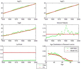
Founda-Fig. 1. Relative individual productivity in the research and economy sector with respect to age

tion 2003, as an indicator of age-dependent productivity in the research sector

wR(a). Figure 1 shows relative productivity of individuals with respect to their age and occupation, as given by these data.

The organization of the economy is decentralized as the interaction between …rms and sectors are through market forces. Individuals decide which sector to work considering expected lifetime wage earnings. Note that although the government subsidies scienti…c activities and venture …nancing, the real econ-omy is still decentralized because it is research institutions, universities and private …rms that carry on research and development.

In order to identify the impact of individual variables, …rst I isolate the social security and education expenditures at the beginning so that I can observe the e¤ect of demographic dynamics on the allocation of labor force. Additionally, in the …rst stage I assume a closed economy model where the country produces technology and goods on its own; but the model can easily be extended to open economy by incorporating immigrants and international capital ‡ows.

3.2 Sectors in the Economy

[image:5.612.161.420.79.304.2]

(6)

Yt =HY t1 At

Z

0

xi;tdi, HY t =

wy(max)

X

a=wy(min)

wY(a)LY t(a) (1)

where LY t(a) is the number of workers at age a and HY t is the human

capi-tal in …nal-good production sector. In the competitive equilibrium labor and intermediate inputs are paid their marginal productivity, i.e.,

wageY;t(a) = (1 ) Yt

HY twY(a); a=ay(min):::ay(max) (2)

pi;t =

HY t xi;t

!(1 )

for ₈i

The intermediate good producing sector is composed of an in…nite number of …rms on the interval [0; At] that have purchased a design from the R&D sector and are monopolists in the production of their particular variety of intermediate good. The only factor of production is capital which is rented at a rate of rt each period and remains without change or depreciation. A …rm that has purchased a design can transform one unit of capital into one unit of intermediate input. Every intermediate …rm then solves the following pro…t maximization problem each period:

maxp(xit)xi;t rtxi;t

Every intermediate …rm acting as a monopolist sets the same price, sells the same quantity of intermediate good and gets the same pro…t:

pit =pt= rt; ₈i (3)

xit =xt =HY t pt

!1=(1 )

=HY t

2

rt

!1=(1 )

; ₈i (4)

it = t= (1 )ptxt= (1 ) Yt

At; 8i (5)

The last equation uses the fact that in equilibrium the output is given byYt= AtHY t1 _xt ₌ _{AtHY t} 2

rt

=(1 )

(7)

Kt=Atxt=AtHY t

2

rt

!1=(1 )

(6)

rt= pt= 2Yt Kt

(7)

Observe that capital is underpaid relative to the competitive case in order to compensate the R&D expenditures. The research sector creates new

de-signs and innovations with the human capital HAt =

ar(max)_P

a=ar(min)

wR(a)LAt(a)

engaged in R&D and current stock of technologyAt. Observe that the level of technology is de…ned as the variety of intermediate goods At. The amount of new designs or equivalently the progress in the technology is given by

At= ( h_At1At)HAt where hAt =HAt in equilibrium. LAt denotes the

num-ber of researchers and ( h_At1At) term de…nes the rate at which R&D labor

force generates ideas. Here hAt captures the negative externalities caused by the ine¢ciency, failure or duplications in the research process. Then the knowl-edge stock evolves according to

At+1 =At+ HAtAt; ; 2(0;1) (8)

Any individual can enter the research sector to search for new designs so R&D labor also receives its marginal productivity:

wageR;t(a) = PA;tH_At1AtwR(a); a=ar(min):::ar(max) (9)

where PA;t is the price of the patent that the research …rm sells to the inter-mediate …rm in each period for production of particular durable.

3.3 Households

The representative household makes the consumption decision in order to maximize life-time utility subject to the budget constraints. Namely,

max Ct

1

X

t=0

t_{(1 +}_nt)t₍ c

1

t

1 ) subject to

(8)

Ct+It =rtKt+ ar(max)

X

a=ar(min)

wageR;t(a)LAt(a)+ ay(max)

X

a=ay(min)

wageY;t(a)LY t(a)+[At t PA;t(At At 1)]

(11)

wherect=Ct=Lt per capita consumption,nt population growth rate between

period (t+ 1) and t, and subjective discount rate. Households’ problem

requires the ‡ow of Ct and PA;t to be

Ct+1

Ct = (1 +nt) [rt+1+ (1 )] (12)

PA;t+1 = [rt+1+ (1 )]PA;t t+1 (13)

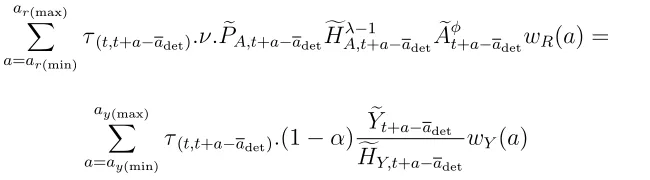
In this decentralized economy labor is engaged only in the R&D and the …nal-good producing sector. At this point I assume that individuals decide which sector to work at certain age adet in their lifetime, and then undergo

a training or education process for each sector with no cost. They become productive after …nishing their sector-speci…c education. Once the individual gives the sector decision , (s)he cannot change the sector later.1 _{The individual}

considers expected discounted wage income throughout his/her lifetime while giving sector decision. In equilibrium, since labor is immobile across sectors, expected discounted wage earnings in both sectors must be equal to each other; otherwise there would be an arbitrage opportunity. Formally,

ar(max)

X

a=ar(min)

(t;t+a adet):wageR;t+a adet(a) =

ay(max)

X

a=ay(min)

(t;t+a adet):wageY;t+a adet(a) for 8t

(14)

)

ar(max)

X

a=ar(min)

(t;t+a adet): :PA;t+a adetH

1

A;t+a adetAt+a adetwR(a) =

ay_X(max)

a=ay(min)

(t;t+a adet):(1 )

Yt+a adet

HY;t+a adet

wY(a) for 8t (15)

1 _{I assumed free entry condition when deriving wage equations in …nal-good}

(9)

(t;t+a adet) =

a_Y1

s=adet

1 qs 1 +rt+s adet

!

(16)

Thus at any time t, the fraction of the cohort at age adet that chooses each

sector is determined by lifetime earnings equality condition. (t;t+a adet) is the

individual discount rate between time period t and t+a adet i.e, between

period at which s/he is at age adet and period s/he is at age a. The discount

rate between consecutive periodst and t+ 1, (equivalently between ageaand

a+ 1) is (t;t+1) = 1₁₊q_ra_t which is a function of interest ratert and probability of

dyingqa at agea. Aggregating one-period discount rates until timet+a adet

yields:

(t;t+a adet) =

a_Y1

s=adet

1 qs 1 +rt+s adet

!

(17)

Finally, labor engaged in two sector for any age cohort should sum up to total employment in that cohort:

LY t(a) +LAt(a) =W orkt(a); a=adet; :::;maxfar(max); ay(max)g (18)

4 Steady-State of the Model

The steady-state analysis allows us to learn the behavior of the system in the long-run. In this section …rst I …nd the steady-state of the population pyramid and then solve for steady-state value and growth rate of variables in the economy.

4.1 Population Pyramid

Population pyramid shows the age-distribution in the society. Let Gt(a)

de-note the percentage of age-group a in the population. If we assume that net population growth rate or total fertility rate2 _{are constant and in addition}

age-dependent mortality rate is constant over time, then the population pyramid of the society de…ned by Gt(a) eventually becomes stable. Let Lt(a) denote

2 _{Total fertility rate (TFR) is the total number of children that a woman would}

(10)

the actual number of people at agea at time t,Lt total population at time t, nt+1 net population growth rate between time t and t+1,qa the probability of

death at the age ofaand T the maximum survival age (qT = 1) The evolution of demographic variables then can be expressed as,

Lt+1 = (1 +nt)Lt (19)

Lt+1(0) =ntLt+ T X

a=0

qaLt(a) (20)

Lt+1(a+ 1) = (1 qa)Lt(a); a= 1; :::; T (21)

Gt(a) = Lt(a)

Lt (22)

The second equation gives the number of new born since increase in the pop-ulation size is equal to new born less of total deaths. In the steady-state

Gt(a) = G(a); nte = n; and Lt = (1 +n)t_L_e

0 That is population grows at

the rate of n and let Lte = Lt=(1 +n)t ₌ _L_e

0 denote the normalized value of

population size. Steady-state age-distributionG(a)e is then

e G(0) = 2 6 6 6 41 +

T X

a=0

a_Q1

i=0(1 qi)

(1 +n)a 3 7 7 7 5 1 (23) e G(a) =

a_Y1

i=0

(1 qi) ! _e

G(0)

(1 +n)a; a = 1; :::; T (24)

f

Lt(a) =G(a)e Lte =G(a)e Le0 (25)

4.2 The Economy

In the steady-state balanced growth, variables grow at constant rate in time. If gX is the growth rate of variable Xt, then Xt = (1 +gX)t_:_Xt:_f _Here _Xt_f ₌ Xt=(1 +gX)t _{is the normalized variable and stationary over time. To …nd the}

(11)

W orkt(a) for di¤erent age groups. I assume labor force participation rate,

total unemployment rateUt and sector-speci…c age-dependent unemployment

rates uA(a); uY(a) to be stable over time. Because labor is immobile across sectors,

LA;t+1(a+ 1)

1 uA(a+ 1)

= LA;t(a) 1 uA(a)

; a ar(min) (26)

LY;t+1(a+ 1)

1 uY(a+ 1) =

LY;t(a)

1 uY(a); a ay(min) (27)

To simplify the solution, I further assume that unemployment rates are equal in research and …nal-good producing sector for all age groups at which both sector employees are working, i.e.,uA(a) = uY(a) =u(a);for max_far(min); ay(min)g

a min_far(max); ay(max)g: This assumption implies

LA;t+1(a+ 1)

LY;t+1(a+ 1)

= LA;t(a) LY;t(a) =

LA;t a+adet(adet)

LY;t a+adet(adet)

; a max_far(min); ay(min)g

(28)

LA;t+1(a+ 1)

W orkt+1(a+ 1)

= LA;t(a) W orkt(a) =

LA;t a+adet(adet)

Lt a+adet(adet)

; a ar(min) (29)

LY;t+1(a+ 1)

W orkt+1(a+ 1)

= LY;t(a) W orkt(a) =

LY;t a+adet(adet)

Lt a+adet(adet)

; a ay(min) (30)

The share of the R&D employment in total employment stays the same over time for the same cohort and equal to the share of individuals who chose R&D sector when they were at the ageadet. Similar result holds for …nal-good

production sector.

At the steady-state, Lt; LY t; LAt; HAt; HAt; W orkt grow at constant rate n. If

we normalizeLt(a); LY t(a); LAt(a)with their growth rates, we get stable vari-ables L(a);e LYe (a); LA(a):e The ratios in equations (29) and (30) now become independent of time and thus,

e LA;t(a) f

W orkt(a) =

LA;t(a) W orkt(a) =

LA;t a+adet(adet)

Lt a+adet(adet)

=mA; a ar(min) (31)

e LY;t(a) f

W orkt(a)

= LY;t(a) W orkt(a) =

LY;t a+adet(adet)

Lt a+adet(adet)

=mY = 1 mA; a ay(min)

(12)

e

LA;t(adet) +LY;t(ae det) =Lt(ae det) (33)

This means that the share of employees in R&D sector inside the workers of that age is the same over all age groups and equal to mA: Likewise the share of employment in …nal-good sector in any age group is mY = 1 mA: Given

population pyramid W ork(a)f and mA, one can calculate steady-state R&D employees in particular age group a.

e LA(a) f

W ork(a) = e

LA(ar(min))

e

L(ar(min))

=mA; ar(min) a ar(max) (34)

e LY(a) f

W ork(a) = e

LY(ay(min))

e

L(ay(min))

=mY; ay(min) a ay(max) (35)

e

LA(a) +LeY(a) = W ork(a)f (36)

At steady-state balanced growth, interest rate is constant over time, rt = r:

To …nd growth rate of variables consider equations (6), (7), (10) and (11),

gY =gC =gI =gK =g (37)

(1 +gY) = (1 +gA)(1 +n) (38)

(1 +gA) = (1 +n) (1 +gA) ₎gA= (1 +n)(1 ) ₍₃₉₎

gPA =g =n (40)

gwageR =gwageY =gA (41)

Scaling variables in model equations and using normalized variables, I obtain the model in terms of stationary variables as

e

Yt=AteHY tf

2

rt

! =(1 )

(13)

f

Kt =AetHfY t

2

rt

!1=(1 )

(43)

(1 +gA)Ate+1 =Ate + HfAtAet; ; 2(0;1) (44)

f HY t =

ay(max)

X

a=ay(min)

wY(a)LY t(a)e (45)

f HAt =

ar_X(max)

a=ar(min)

wR(a)LeAt(a) (46)

ar(max)

X

a=ar(min)

(t;t+a adet): :PA;te +a adetHf

1

A;t+a adetAet+a adetwR(a) =

ay(max)

X

a=ay(min)

(t;t+a adet):(1 )

e

Yt+a adet

f

HY;t+a adet

wY(a) (47)

e

LY t(a) +LAt(a) =e W orkt(a);f a=adet; :::;maxfar(max); ay(max)g (48)

(1 +g)Ktf+1 = (1 )Ktf +Ite (49)

e

Ct+Ite =rtKt+f ar(max)

X

a=ar(min)

e

wageR;t(a)LAt(a)+e ay(max)

X

a=ay(min)

e

wageY;t(a)LY t(a)+e "

e

Atet PA;t(e Ate e At 1

1 +gA) #

(50)

e_t = (1 )Yte e At

; ₈i

rt= 2 e Yt f

Kt (51)

(14)

(1 +gC)

e_Ct₊₁ e Ct

!

= (1 +n) [rt+1+ (1 )] (53)

At the steady-state,Xtf+1 =Xtf =Xssf =X;f 8t so given model parameters and

the data for labor force participation rate and age-dependent unemployment rate, I compute the decentralized steady-state values with the above formulae.

5 Calibration of The Model

As an empirical application, I attempt to …t the model to the United States data and compute model parameters. I choose United States since the model assumes the country producing its own technology. The equilibrium outcome of the model heavily depends on the choice of parameters, so calibrated para-meters are helpful to understand the economy and perform forecast.

5.1 Calibration Method

Based on the availability of data, the model is calibrated using 1950-2000 data, and variables are predicted for the period 2001-2050. The period is one year and the …rst period is 1950. There are 8 parameters to calibrate:

; ; ; ; ; ; ; with constraints ; ; ; ; ₂(0;1) and ; ; >0. Data for wY(a) and wY(a) de…nes productivity relative to age groups but not in absolute terms. Thus the last parameter multiplieswY(a)data to obtain the absolute value. Since multiplieswR(a) in (8) an additional parameter is not required.

I calibrate the model so that its steady-state matches the statistics of the US data. First we need to …nd values of exogenous variables. ForLe andn;I regress United States total population 1950-2000 assuming population growth rate is constant. I use time-average of 1960 to 2000 age-speci…c labor force participa-tion rate and age-speci…c unemployment rate to calculate W orkf variable.

Observable endogenous variables of the model areYt; Ct; It; rt; LY t; LAt. I choose target values of calibration as gY; Y ;e C;e I; r:e I perform log-linear regressions on data to …nd the growth rate and intercepts gY; Y ;e C;e I:e Observe that I chose growth rate of Yt as the growth rate g of the model. Interest rate r

(15)

calibration because the share of R&D employment in total employment has not stabilized in the period.

There are 8 parameters but 5 statistics to match, thus I need to set 3 of the variables. Following the convention in the literature, I use = 0:33; = 0:995

and = 0:05:Demographic parameters are maximum age T = 90 and sector decision age adet = 18: Scientists, engineers and technology labor force are

productive between age ar(min) = 25 and ar(max) = 85: Workers in …nal-good

production sector are productive between ageay(min) = 20 and ay(max) = 65:

[image:15.612.92.531.428.477.2]

5.2 Calibration Results

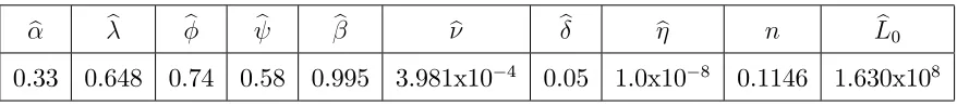
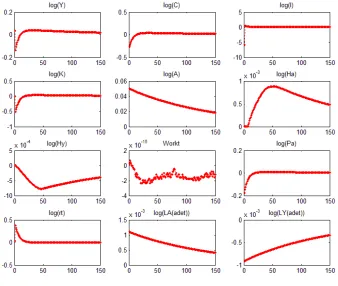
Table 1 shows the estimated parameter values, corresponding steady-state of the model and the target statistics in the data. Fitted variables are, then computed via their growth rate and steady-state value. Figure 2 plots actual time series data together with the …tted variables from 1950 to 2005. The …gure also shows the age distribution of R&D employees in NSF Integrated Database 2003. In this respect the model prediction of R&D workforce age distribution is close to the actual data. Note that according to model the share of R&D employment in total employment is %45:32; while in reality it is never above

%6 (although increasing). This is due to the fact that labor force allocation has not reached its steady-state and there is an inertia in labor force.

b b b b b b b b n Lb0

0.33 0.648 0.74 0.58 0.995 3.981x10 4 _{0.05 1.0x10} 8 _{0.1146 1.630x10}8

Table 1: Optimum parameter values for the model

6 Assessing Steady-States

(16)

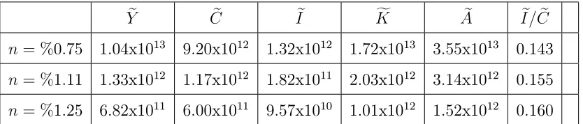
In the …rst case, I use the same set of coe¢cients as in the …rst one, except I choose a lower steady-state population growth rate: n = %0:75: In the sec-ond case, I choose a higher steady-state population growth rate: n = %1:25:

Thereby, one can observe the change in steady-state values and growth rates in the models. The steady-states of the model is tabulated for di¤erent popu-lation growth rates in Table 2.

e

Y Ce Ie Kf Ae I=e Ce

n= %0:75 1:04x1013 _9:20_x₁₀12 _1:32_x₁₀12 _1:72_x₁₀13 _3:55_x₁₀13 _0:143

n= %1:11 1:33x1012 _1:17_x₁₀12 _1:82_x₁₀11 _2:03_x₁₀12 _3:14_x₁₀12 _0:155

n= %1:25 6:82x1011 _6:00_x₁₀11 _9:57_x₁₀10 _1:01_x₁₀12 _1:52_x₁₀12 _0:160

f

W ork LA=e W orkf LYe =W orkf PAe r gY =g gA

n= %0:75 7:83x107 _0:642 _0:358 _7:74 _%6:59 _2:64_x₁₀ 2 _1:88_x₁₀ 2

n= %1:11 7:50x107 _0:453 _0:547 _9:34 _%7:13 _3:95_x₁₀ 2 _2:80_x₁₀ 2

[image:16.612.92.509.222.311.2]

n= %1:25 7:37x107 _0:407 _0:593 _9:33 _%7:32 _4:43_x₁₀ 2 _3:14_x₁₀ 2

Table 2: Steady-state values and growth rates for di¤erent population growth rates. The model parameters are = 0:33; = 0:648; = 0:74; = 0:58; = 0:995; = 3:981x10 4_; _{= 0:05;} _{= 1:0}_x₁₀ 8_:_{Population intercept}_L_e _{= 1:63}_x₁₀8_:

As seen in the table, growth rate of model variables increase as population growth rate increases. Population growth thus fosters economic growth and rate of technological progress in the steady-state. Higher population growth rate, however, results smaller steady-state value (intercept) forY ;e C;e I;e K;f Ae

because population involves more young members and ratio of labor force to total population is lower. However when population is growing faster, house-holds prefer to invest more portion of their income because they bene…t from higher output growth rate in the future.

(17)

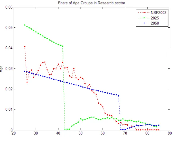
Figure 3 shows the age-distribution among the employees of the R&D sector for the three cases. The resultant distributions are similar. Note that when population growth rate is lower, the research sector is relatively older because the population consists of more old members.

7 Impulse Response

Since fertility and technological progress are inherently random, it’s reasonable to de…neAt and Gt(a) as stochastic variables. This enables us to understand response of the demographic multisector economy against shocks. With this modi…cation, the dynamic equations become

(1 +gA)Ate+1 =Ate + HfAtAet +"A; ; 2(0;1) (54)

e

Gt+1(a) =Get(a) +"G(a); a= 0; :::; T (55)

where"Aand"G(a)are technology and demographic shocks respectively. Here we (distort) apply one-period shock to the system at time t when it was in steady-state previously. Thereafter the population pyramid and the economic system react to shocks and eventually return to steady-state after some tran-sitional period. We can apply one type of shock or both shocks together.

To get the impulse response, we need to …nd the state transition equation. I achieve this using log-linear approximation of the dynamic equations. Note that we cannot use the original deterministic system of dynamic equations becauseAetandGet(a)are now stochastic, thus equation (44) should be replaced

with the new stochastic Ate equation (54). Furthermore, the Euler equations now turn into expectational equations, in particular expectation operator is introduced to the right-hand side of equations (52) and (53).

Note that the number of people choosing R&D sector and …nal-good produc-tion sector at each period of time are implicitly given by the equaproduc-tion (47) stating equality of lifetime discounted wage earnings among sectors. In order to perform log-linear approximation of model equations, I …nd explicit formula for number of people choosing each sector at decision age cohortLA;t(ae det)and

e

LY;t(adet) in terms of other model variables. For this I approximate the

pol-icy functionLA;t(ae det)with Chebsyhev polynomials and determine its optimal

(18)

Having explicit form of policy functions, I obtain the following state-transition equation by log-linear approximation:

A:ext+1 =B:ext+C:#t+1+D:"t+1 (56)

where A and B are state matrices andxte is the state vector including variables

e

yt;ect;eit;ekt;eat;elt;ehAt;hY t;e workt;e pAt;e et;rt;e elAt(a); a =adet:::ar(max)andelY t(a);

a = adet:::ay(max): Note that the state vector consists of logged deviations of

normalized variables from their steady-state.#t+1is the vector of expectational

errors and"t+1 is the composite vector that carries structural shocks and

time-dependent values of exogenously determined variables W orktf and Lte . The structural shock "A to Ate is now in terms of standard deviation of Ate (since we use logged deviation of Ate from steady-state in the state vector) while demographic shock "G(a) is still in its absolute value. Using Sim’s solution method, we get the evolution of state as

e

xt+1 =F:ext+H: t+1; t 0 (57)

whereF is the state transition matrix and t+1 is as de…ned before. In the …rst

experiment, I choose the original set of parameters in calibration and apply only a technology shock of "A = 0:05; that is 5 percent standard deviation shock. In the second experiment I use the same set of parameters but apply a 10 percent demographic shock to the cohort at ageadetto see the impact more

clearly. That is I apply"G(adet) = 0:10G(ae det)and then scale Gt(a)e properly

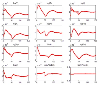
(so that it adds up to 1). The impulse response of economy are shown in …gure 4 and 5 in the Appendix C. Shocks are applied at t = 0 when the system is at steady-state3_.

The …rst observation is that even if a relatively small amount of "G(adet)

shock to single cohort has been applied, it takes more than hundred years for population pyramid to stabilize. If the demographic shock"G(a)was applied to more than one cohort, the population pyramid would stabilize in longer time period. This also causes other variables to return to steady-state in a long period of time. Therefore demographic economic models have very long time-horizon, and in practice they never reach their steady-state because technology shocks are frequent and population growth rate is not constant in the long-run. Other factors like war or disease may further alter the age distribution in the society.

3 _{Because the space is limited, I can only show several samples of}_G_e

tresponse. The

(19)

The impulse response to the technology shock is relatively smooth whereas impulse response to the demographic shock has ‡uctuations and irregulari-ties. As far as the amplitude is concerned, variables show greater response to the technology shock "A compared to the demographic shock, as the demo-graphic shock is applied to single cohort. The impact of the demodemo-graphic shock however is more durable and the variables show variations above and below their steady-state. The exception is that it takes longer for At;e LA;t(ae det)and

e

LA;t(adet)to return to their steady-state in reaction to the technology shock.

8 Forecasting Economic Growth

After calibrating the model and …nding evolution of the economy, I make pre-dictions for TFP growth of United States to observe the impact of population ageing. I forecast the model from year 2001 to 2050. I use the set of para-meters obtained in calibration. I take Lt; Gt(a); W orkt and nt as exogenous. Since there is no data for annual employment forecast up to 2050 for United States, I use year 2000 data for age-speci…c labor force participation rate and unemployment rate.

At each time period t, given present values of state variables Kct;Abt;PbAt; c

HAt; HY t;c one can compute the choice variables Ct;b It;b LAt(ab det);LY t(ab det)

using intratemporal optimization conditions. Number of people at the age of

adet at time t choosing R&D sector LbAt(adet) is computed using Chebshyev

function derived in the previous section. Calculation of the Chebshyev func-tion is explained in the Appendix. The other sector decision then becomes

b

LY t(adet) =W orkt(adet) LAt(ab det):Having time t choice variables, next

pe-riod state variablesKtc+1;Atb+1;PA;tb +1;can be estimated using state transition

equations. Knowing LAt(a); ab = adet:::ar(max) and LY t(a); ab = adet:::ay(max) I

compute human capital in the next period HA;tc +1; HY;tc +1. Forecasting

proce-dure then continues with the next period and so on. Note that capital and knowledge stock in the …rst period of forecast (year 2001) are evaluated using …tted variables Kc2000, Ab2000 and year 2000 investment data. I obtain initial

age-distribution in the R&D sector from National Science Foundation Inte-grated Database 2003. I evaluate share of age groups among those employees who are in the research and development category in the database.

Figure 6 in Appendix C shows actual data from 1950 to 2000 with the fore-casted variables from 2001 to 2050. Logged values are plotted to see the change in growth rates. Note that actualAt andKt are unobservable, so …tted values

b

(20)

Observe that there are discontinuities in Ytb and Itb in year 2000. One expla-nation for the discontinuity between the data and the forecasts is that the economy has not reached its steady-state, especially share of employment in science, technology and engineering sectors. Decreasing population growth rate and variations in population pyramid over time are also reason for the disconti-nuity. Besides one may argue that the actual consumption rate is greater than its steady-state value. Note that the model predicts lower HY tc value than the actual data because approximately % 95 of employees work in economy-wide sector in 2000 while this ratio for the model is %54.7. So forecasted human capitalHY tc decreases over time which causes interest rate also to decrease. Be-cause interest rate is decreasing, the model then predicts consumption growth to slow down and then total consumption to decrease.

Figure 7 depicts the age-distribution forecasts in the R&D sector for 2025 and 2050. Because ratio of people choosing science sector LAt(ab det)=Lt(ab det);

is increasing, labor force in research sector will be relatively younger in 2025 compared to 2003. Age-distribution will be closer to its steady-state distribu-tion in 2050.

9 Discussion and Further Research

Demographic economy models are powerful to study the relationship between society, total factor productivity, economic output and sectors as the mod-els employ population pyramid to estimate labor and population variables in detail. One can extend the model by endogeneouzing population growth, for instance Becker and Lewis (1973) model can be used to determine the fertility choice. In addition social security expenditures and (possibly sector-dependent4_{) educational cost can be added. The social planner in this case}

also considers training costs while allocating the labor force between sectors. Similarly individuals in the economy can consider training costs while choosing their sector. Introducing social security expenditures makes the model more realistic and promising since health expenditures and needs of old people will become signi…cant as population ages. Note that although promising, the ed-ucational and social security expenditures will make the model more compli-cated and more parametric. Furthermore, data for these variables are available only for recent years. Another extension is open-economy model where migra-tion and internamigra-tional capital ‡ows are allowed. But since immigrants bring their own human capital, the model environment should be modi…ed to adapt immigrant pro…les. Finally, demographic pro…le of OECD countries, China, Japan and global economic equilibrium, similar to Fehr, Jokisch and Kotliko¤ (2005) is a potential long-term project.

(21)

10 Conclusion

In this paper I have founded the basis of demographic economic growth mod-els and thus established a framework in which the impact of age-distribution of the society on economic growth can be examined. The way demographic structure in‡uences economy is through age-dependent productivity and en-dogenous allocation of individuals between sectors. In the model, there are three sectors in the economy, wages and market forces determine the alloca-tion. Higher population growth provides greater economic growth and faster technological progress. As an empirical application I …t the model to United States data for 1950 to 2000, and perform 50 year forecast to see the impact of population ageing. Technological progress seems to be sustainable despite population ageing. The size and the share of employment in the R&D sectors will continue to rise. Aside from the model presented in this paper, there are other forces such as social security or education expenditures by which pop-ulation ageing may enhance or suspend economic growth. These extensions may be the topic of subsequent papers.

11 Data and Sources

(22)

to calculate age-distribution inside R&D sector with interpolation.

Acknowledgements

This research is funded by University of Pittsburgh, Department of Economics. I am grateful to Marla Ripoll and David Dejong for their supervision to my project. Special thanks to Thomas Rawski and Spring 2008 Economic Writing course participants for their feedback.

References

[1] Becker G.S. and Lewis H. G., 1973. “On the interaction between quality and quantity of children”, Journal of Political Economy 81, pp 279-288

[2] Bratsberg, B., Ragan J. F. Jr. and Warren J. T., 2003. “Negative Returns to Seniority: New Evidence in Academic Markets.”, Industrial and Labor Relations Review 56(2), pp. 306-323.

[3] Caldwell J., 1976. “Toward a restatement of demographic transition theory”, Population and Development Review 2, pp 321-366

[4] Cutler D., Poterba J., Sheiner L., Summers L. and Akerlof G., 1990. “An Aging Society: Opportunity or Challenge?”, Brookings Papers on Economic Activity 1990(1), pp 1-73.

[5] D’Albis H., 2007. “Demographic structure and capital accumulation”, Journal of Economic Theory 132, pp 411-434

[6] Dejong D, Dave C., 2007. "Structural Macroeconometrics", Princeton University Press, Princeton.

[7] Domeij D. and Floden M., 2006. “Population Aging and International Capital Flows” International Economic Review 47, pp 1013-1032

[8] Federal Reserve Bank of St. Louis, Online Economic Data. http://research.stlouisfed.org/fred2/

[9] Fehr H., Jokisch S. and Kotliko¤ L., 2004. “The role of immigration in dealing with the developed world’s demographic transition” NBER Working Paper no 10512

(23)

[11] Hansen G. D., 1993. "The Cyclical and Secular Behaviour of the Labour Input: Comparing E¢ciency Units and Hours Worked", Journal of Applied Econometrics 8, pp 71-80

[12] Jones Charles I., 1995. “R&D-Based Models of Economic Growth” Journal of Political Economy 103(4), pp 759-784

[13] Jones, Charles I., 2004. “Growth and Ideas” NBER Working Paper No. W10767 [14] Kremer M., 1993. "Population Growth and Technological Change: One Million

BC to 1990", Quarterly Journal of Economics 108, pp 681-716

[15] Miles D., 1999. “Modelling the Impact of Demographic Change Upon the Economy” The Economic Journal 109, No. 452, pp 1-36

[16] National Science Foundation SESTAT Online Database. http://www.nsf.gov/statistics/sestat/

[17] OECD Stat Online Database. http://stats.oecd.org/WBOS/Index.aspx?QueryName=451&QueryType=View [18] Sims, Christopher A., 2001. "Solving Linear Rational Expectations Models".

Computational Economics 20, pp 1-20.

[19] Stephan, P. E. and Levin S. G., 1988. “Measures of Scienti…c Output and the Age-Productivity Relationship.”, Ch. 2, in Anthony Van Raan, ed., Handbook of Quantitative Studies of Science and Technology, Elsevier Science Publishers, pp. 31-80

[20] World Population Prospects: The 2006 Revision Population Database. http://esa.un.org/unpp/

[21] World Population Prospects: The 2006 version, Highlights. United Nations, New York; 2007.

12 Appendix.

12.1 Appendix A: Nonlinear Approximation of Policy Function

The policy function I seek for sector decision variable is of 2nd _{order (r=2)}

(24)

e

LA;t(adet) = 1+ 2T1(esAt) + 3T1(esPAt) + 4T1(esKt) + 5T1(esHAt) (58)

+ 6T2(esAt) + 7T2(esPAt) + 8T2(esKt) + 9T2(esHAt)

+ 10T1(esAt)T1(esPAt) + 11T1(esAt)T1(esKt) + 12T1(esAt)T1(esHAt) + 13T1(esPAt)T1(esKt)

+ ₁₄T1(esPAt)T1(esHAt) + 15T1(esKt)T1(esHAt) + 16T1(esAt)T1(esPAt)T1(esHAt)

where 1::: 16 are parameters to estimate and

Tj(esXt) = cos(j:cos 1_(e_s

Xt)); seXt =

f

Xt Xfss !_X_e

e

sXt is a measure of deviation ofXtf variable from its steady-state with respect

to a range !_X_e. If Xft varies !_X_e=2 units above or below its steady-state then e

sXt is a transformation of Xtf to [-1, 1] scale. Here I set !_Xe = 4 _Xe i.e., I

assume Xtf lies in its 4 standard deviation range.

With this equation for LA;t(ae det) and given candidate parameters, the

dy-namic system is ready to solve. For this I de…ne the state vectorxetcomposed of

variablesyt;e ct;e eit;kt;e at;e elt;ehAt;ehY t;workt;e pAt;e et;rt;e lAt(a); ae =adet:::ar(max)

and elY t(a); a = adet:::ay(max): Note that the state vector consists of logged

deviations of normalized variables from their steady-state. Log-linear approx-imation of the state vector around its steady-state yields the state transition equation:

A( ):ext+1 =B( ):ext+C:#t+1+D:"t+1 (59)

whereA( ) andB( )are state matrices (depending on the choice of

parame-ters).#t+1 is the vector of expectational errors and"t+1 is the composite vector

that carries structural shocks and time-dependent values of exogenously de-termined variablesW orktf andLte . The structural shock "AtoAte is in terms of standard deviation ofAet(since we use logged deviation ofAetfrom steady-state

in the state vector) while demographic shock"G(a)is still in its absolute value. I solve this dynamic stochastic linear system using Sim’s solution method and get the evolution of state as

e

xt+1=F( ):ext+H( ): t+1; t 0 (60)

where F( ) is the state transition matrix. Thereafter I determine the future

(25)

sectors, mentioned in the text, holds: Thus ₁::: ₁₆ parameters should be chosen so as to In the …rst experiment, I choose the original set of

ar(max)

X

a=ar(min)

(t;t+a adet): :PA;te +a adetHf

1

A;t+a adetAet+a adetwR(a) =

ay(max)

X

a=ay(min)

(t;t+a adet):(1 )

e

Yt+a adet

f

HY;t+a adet

wY(a) (61)

At this point, Chebyshev interpolation theorem helps us to …nd the desired parameters. According to the theorem, if the Chebyshev function is zero at the roots of rth _{order polynomial} _Tr(e_sX

t);then the function is close to zero on

the whole sXe t domain. The roots of the r

th _{order polynomial}_Tr(e_s) _are

b

sj = cos 2j 1

2r j = 1;2; :::r (62)

In this problem r=2 and the roots of T2(esXt) polynomial are sjb =

p

2=2 and

b

sj = p2=2 for each variableXtf = At;e PAt;e Kt;f HAtf . With two roots of each four variable, there are 16 possible combinations of roots. The objective is to choose ₁::: ₁₆ so that condition (61) is satis…ed at each 16 combination

of the Chebyshev roots. In the programming stage I …nd the parameters

using Matlab’s fminsearch routine. The optimum parameters of the Chebyshev function turns out to be:

1 2 3 4 5 6 7 8

1:165x106 _1:878_x₁₀2 _2:864_x₁₀ 4 _8:613_x₁₀ 10 _1:55_x₁₀ 2 _2:51_x₁₀3 _4:836_x₁₀ 8 _3:743_x₁₀ 19