Interactive computer graphics in non-linear optimization.
GHARIB, Sheida.Available from Sheffield Hallam University Research Archive (SHURA) at: http://shura.shu.ac.uk/19683/
This document is the author deposited version. You are advised to consult the publisher's version if you wish to cite from it.
Published version
GHARIB, Sheida. (1979). Interactive computer graphics in non-linear optimization. Masters, Sheffield Hallam University (United Kingdom)..
Copyright and re-use policy
See http://shura.shu.ac.uk/information.html
Sheffield Hallam University Research Archive
Sheffield City Polytechnic Eric M ensforth Library
REFERENCE ONLY
This book must not be taken from the LibraryPL/26
ProQuest Number: 10696982
All rights reserved
INFORMATION TO ALL USERS
The quality of this reproduction is dependent upon the quality of the copy submitted.
In the unlikely event that the author did not send a com plete manuscript and there are missing pages, these will be noted. Also, if material had to be removed,
a note will indicate the deletion.
uest
ProQuest 10696982
Published by ProQuest LLC(2017). Copyright of the Dissertation is held by the Author.
All rights reserved.
This work is protected against unauthorized copying under Title 17, United States C ode Microform Edition © ProQuest LLC.
ProQuest LLC.
789 East Eisenhower Parkway P.O. Box 1346
INTERACTIVE COMPUTER GRAPHICS IN
NON-LINEAR OPTIMIZATION
by
SHEIDA GHARIB
Being a thesis submitted to the Council for National Academic Awards in partial fulfilment of the requirements for the Council's degree of
Master of Philosophy
Sponsoring establishment: Sheffield City Polytechnic Collaborating establishment: University of Bradford
ACKNOWLEDGEMENT
The author wishes to express her thanks to her supervisors. Thanks are especially due to Dr I Cooper who has given valuable and constructive advice, and encouragement during the course of the study. The help received from Dr G F Raggett and Dr J Stephenson (University of Bradford) and Dr B G Hutley (Chemistry) is also acknowledged.
The author would also like to express her gratitude to the staff of Sheffield City Polytechnic Computer Services department.
Thanks are due to the Optimization Centre of Hatfield Polytechnic who contributed some ideas and material in the early stages of the project.
Finally the author is indebted to Mrs C J Barker for her skilful typing of this thesis.
ABSTRACT
S Gharib - "Interactive Computer Graphics in Non-linear Optimization"
The thesis surveys the current state of knowledge in the field of both interactive computer graphics and non-linear optimization.
The potential contribution of interactive computer graphics in non linear optimization is then evaluated from the points of view of model formulation and solution, and the requirements of an interactive system for realizing this potential are outlined.
Such a system is developed and described, together with a full account of its applications to both real and standard test problems. A novel application is the direct optimization of N-dimensional (N > 2) problems by visual analysis of 1 and 2 dimensional sub-problems, following on the formal development of an algorithm for this approach. The inter active control of conventional methods through computer graphics is also featured.
CONTENTS Page
ACKNOWLEDGEMENT (i)
ABSTRACT ( ii)
CHAPTER ONE: Interactive Computer'Graphics 1
1.1 The Evolution of Computer Graphics 1
1.2 The Elements of Interactive Computer Graphics 4
1.3 Applications of Interactive Computer Graphics 14
1.4 The Design of Interactive Computer Graphics Systems 17
1.5 Summary 20
CHAPTER TWO: Non-1inear Optimization 22
2.1 Preliminary Aspects of Optimization 22
2.2 Mathematical Models 23
2.3 Local and Global Optima 24
2.4 Classification of Objective Functions 25
2.5 Methods of Optimization 25
2.6 Comparison of Algorithms 37
CHAPTER THREE: Interactive Computer Graphics in Optimization 39
3.1 Interactive Computer Graphics in Optimization 39
3.2 Evaluation of Potential 40
3.3 System Requirements 42
CHAPTER FOUR: An Interactive Computer Graphics System for
Optimization _ 44
4.1 Hardware Mechanism 4-4
4.2 Software 45
CHAPTER FIVE: Applications to Test Problems
5.1 Problems in One-dimension 5.2 Problems in Two-dimensions 5.3 Problems in N-dimensions 5.4 Plane Analysis Method
CHAPTER SIX: A Practical Application 6.1 Molecular Vibrational Analysis 6.2 Minimization Problem
6.3 Methods of Solution 6.4 Comparison of Methods
CHAPTER SEVEN: Appraisal and Conclusion
APPENDIX
REFERENCES
CHAPTER ONE
Interactive Computer Graphics
/ — :
---In this chapter some of the general principles concerning the history, applications and design of interactive computer graphics systems are discussed.
The introductory section presents the origin and the development of graphical techniques. In the following section, the facets of hardware and softv/are for interactive graphics are considered.
An account of some of the application areas of interactive graphics and the merits of graphical computing methods is given in the next
section. Finally, in the last section of this introductory chapter, some specific factors relating to the design of an interactive graphics system are considered.
1.1 The Evolution of Computer Graphics
The need for increased calculating power to solve complex scientific problems gave rise to the invention of computers. Since their invention, over thirty years ago, computers have been closely linked to the developments of many scientific and engin eering methods. Until the late 1940's computers were only capable of producing numerical results, using a high speed line-printer. However, it was found that these numerical results were not suffi cient when dealing with empirical quantities and data exhibiting com plex relational attributes. It was fe lt that some numerical results could be more meaningful if presented in graphical forms rather
-• than tabular forms. There are several reasons for this assertion, (i) Graphical illustrations are easier to understand, specially
i f the user is looking for comparison or trends in large files of output data. In subject areas such as statistics, computer-produced tabulations are used as raw data to produce graphical presentation of data. These graphs are useful aids to the detection of errors in large input data file s.
( ii) When presenting the output graphically, there is more fle x i b ility in the showing of emphasis on key areis.
( i ii ) The graphs are more compact, since many pages of numerical output' can be contained in a few graphs.
(iv) .Data can be seen in two dimensions as opposed to a one dimen sional lis t of figures. This is particularly useful for showing relationships between variables, allowing a better interpretation of the data.
It was only natural that there would soon be a demand for the computer to be able to communicate its results in a graphical form whenever appropriate. However, technology has not allowed this feature to develop at so rapid a rate as the manipulation of numeri cal data, and it was not until 1953, that the Benson-Lchner
Corporation introduced a digital graph-plotter. Graph-plotters operate slowly when compared with general computer processing. They are largely used in the place of manual graph plotting, which means that the graphical operation is a passive one, and is thus usually referred to as non-interactive graphics. The graph-plotters are distinctly inefficient when a sequence of further computation
-depends upon the analysis of the displayed graph, and this draw back has led to the development of specialised equipment which enables the graphing operation to be performed under interactive control.
Interactive computer graphics can be defined as a close interaction between the user and the computer through the use of a visual display, an input device, and a special computer language. The user is able to communicate with the computer and to receive a direct response r. om it . This two way conversation may be of a graphical or pictorial nature, and, as a result of previous pro gramming, the computer can analyse the output, perform calculations, and almost instantaneously present a revised display for further analysis if required.
The pioneering work in the field of interactive computer graphics was carried out by the US Air Force. In the early 1950's a system called SAGE (1), Semi Automatic Ground Environment, was designed in order to help to protect the United States from sur prise air attacks. SAGE became operational with one computer centre in 1958 and has now been used in many centres.
SAGE presented visual information on aircraft positions, and the air force personnel could communicate with the computer using a light pen. This system laid the foundation for further hardware and software developments in the field of interactive computer graphics.
In 1962, Sutherland and Johnson (2), announced the development of a system known as 'Sketchpad', at M.I.T.
-In parallel with Sutherland's work on sketchpad, research was being carried out in industry mainly at General Motors (3), and Itek Laboratories (4).
In 1959, with a contribution made by IBM, General Motors produced DAC-1, 'Design Augmented by Computer', a computer aided design system for the automobile industry. The Itek Laboratories were also involved in developing an on line graphics system for lens design. This system was based on the laboratory's early research work on graph plotters.
The systems mentioned so far had two bothersome characteris tics in common;
(i) the hardware was expensive
( ii) the software used a great amount of time.
By the early seventies, there had been further hardware develop ments leading to the improved interactive computer graphics systems which are being used by industry and research establishments today. These developments include the emergence of the storage tube, the micro processor and satellite computers, aiming to provide more computing power at substantially reduced costs, and hence more effective computer graphics.
Modern systems are usually described in terms of their hard ware configurations, and their software needs and capabilities. These will be briefly discussed in the following section.
1.2 The Elements of Interactive Computer Graphics
This section briefly describes the hardware and software currently available generally for use in interactive graphics systems.
-1.2.1 Interactive Graphics Systems
There are two main types of interactive graphics installa tion in common use
-(a) Stand-alone system (b) Time-sharing system (a) Stand-alone System
A typical system of this type would consist of a processor with 8k words, a visual display, and a graphical input-output device. The software of such a system is compact, yet fairly complex, frequently written in assembly language or even machine code.
This type of system can be used for applications which require little processing power. It offers the advantage of rapid personalised data processing, particularly when it possesses interactive features.
Many such systems exist, and perform useful jobs in industrial laboratories and research establishments. (b) Time-sharing System
This type of graphics installation provides graphics terminals as part of a general time-sharing system. This system can be useful for applications which require the computer to perform extensive calculations under the control of the user. The processor in such a system is normally available for non-graphical applications, although it can support graphical applications.
-The system used for the development of the project which forms the central part of this thesis is a time sharing system. It consists of an IBM/370 main computer, linked to a Tektronix 4014 graphics terminal. The display file is held in the core of the main computer, where the display controller had access to it.
The main difficulty which arises with operating a time sharing system is that each user receives services only
intermittently. A user with a display however, requires that the display should be animated continuously, and that for
certain services, the user should receive instantaneous response. These conditions can best be met i f the display file
is driven by a small computer connected as a satellite to a time-sharing system. Such arrangement does offer several distinct advantages:
1. It provides an independent source of computing power. 2. Allows the fle x ib ility of choosing the position of the
equipment.
3. It can act as a concentrator for multiple display consoles. 4. It can operate as a stand-alone system without interrupting
the host computer for servicing.
The main disadvantage of host-satellite systems is that experience in their use is relatively limited, and i f the satellite is situated remotely from the host, program develop ment can produce problems. Furthermore, i f either the link or the host computer fa ils , the system is normally unuseable.
-Thus, when there are doubts about the effectiveness of a satellite system, then either.a stand-alone or a conven tional time-sharing system with display unit can be con sidered to be better suited alternatives. However, contin uing developments of graphics facilities allied to micro computers may eventually swing the balance in favour of the stand-alone system for virtually all types of application, other than those involving major computations.
1.2.2 Hardware
An interactive computer graphics terminal is usually struc-. tured as an extension of a large computerstruc-. The basic elements of
grpahics hardware are -Display Channel Display Controller Display Console Input Devices
The function of this hardware is to allow application programs to use the display unit for graphical output, while running in the central processor unit.
A complicated picture will call for a long lis t of data and character descriptions. The graphical display instructions, the data containing the picture, or the result of an analysis can all be stored in the display file . The display file is continuously accessed by the display channels and graphical commands are sent to the display controller. This has two main advantages. First,
-the display channels become much simpler devices, as -the computer does not have to refresh them regularly. Second, the load on the computer can be reduced by increasing the fle x ib ility of the display controller to handle some of the graphical instructions. This effectively changes the display controller into a small computer its e lf, called the display processor.
To produce a continuous picture the display processor reads the display file , and executes the operations required to, display the picture, and refreshes it as often as fifty times a second.
Interactive computer graphics consoles require at least one input device for use in conjunction with the display. A keyboard is essential so that alphanumeric information can be entered, but it is also necessary to have some means of transferring geometrical information to the computer.
There are two ways for passing geometrical information to the computer,
(i) pointing ( ii) positioning
The light pen is one of the pointing devices which is more commonly used. It has the advantage over the other input devices in that its positional data is determined by the program, and it does not depend on any physical measurements of the actual pen position. The disadvantage of the light pen is that i t is very sensitive to surrounding illumination, and it cannot be con veniently used with the storage tube.
-The joystick, trackball and cursor are positioning devices, and they do use the screen directly. A more recent development in this field is the 'MOUSE' (5), produced by the Stanford Research Institute. All these devices operate on the principle of moving a control to pass two-dimensional information to the computer.
The input device used in the project described in this thesis is the cursor. Two crossed lines appear on the screen, by the user's request, and the co-ordinates of the point of interaction of the two lines can be recorded. The two lines can be repositioned by thumb-wheel when the co-ordinates of a new point are required.
.2.3 Software
In a computer graphics system, the software produces an interface between the computer and the graphics devices. There are three fundamental components in the software
-(i) The executive
( ii) The applications programs ( i ii ) Graphics software
(i) The Executive
This part of the software attempts to blend the best features of the hardware, the applications programs and the user in such a way that the user can interact in a harmoniou dialogue with the computer. The executives are usually supplied by the computer manufacturers, and most of them are
-not graphics oriented, since they control all other programs running in a computer system. In a multi-terminal computer system, the executive is responsible for the sharing of time between all the terminals attached to the drive pro cessor.
( ii) Applications Programs
The applications programs are similar to the problem-oriented programs in a batch system with the difference that they run in real-time. They specify what is to be displayed by producing definite commands or constructing a data struc ture representing the picture. The amount of structuring used by the applications programs to describe a picture depends entirely on the applications. If no particular structure exists, the picture will be described in terms of co-ordinates.
In general, a graphical system contains three groups of data
-(a) the data base for the applications programs (b) the data structure representing the display (c) the data for the display file
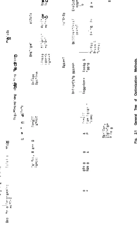
In many systems the display file is combined with the display structure.Figure 1.1 shows the data path through a typical graphics system.
The commands in the applications programs are written in a high level language which must be able to program the applications, and to handle the graphics devices.
-" O .c
fd 0
• r —
-cr CL
fO S -CT>
1 C o
Transformation Co-ordinate
Data
display f il e
Input
recognition
Applications Program
Display
2-D Transformation
Graphical data input
Generation of display code Non-graphical
output
Transformation of an application term to geometric term
Fig. 1.1 Data Path Through A System.
11
FORTRAN is the most commonly used language in computer graphics. The main reason for this is its wide range of scientific applications, and also because on many small and medium size computers i t is the only language used. Unfor tunately, FORTRAN, has weaknesses. I t gives no programming structure, and its subroutines and functions are non
recursive. The usage of its 'DO LOOP' and 'IF ' statements is limited but i t has the advantage of completing a task more rapidly than an equivalent program written in another high level language.
ALGOL 68, PL/1, BASIC and JOSS are some of the other high level languages used for computer graphics. The last two languages mentioned are conversational, but because of their limited data structure fa c ilitie s are only suitable
for informal problem solving. For the present time, however, APL remainsthe only conversational language suitable for complex problem solving using graphics.
A more recently developed language for computer graphics is EULER. This language is designed by Wirth (6 ), as a generalisation of ALGOL 60. The program structure fa c ilitie s
of this language are very powerful and i t is a language of
free type declaration.
In general, some of the high level languages have fa c ilitie s for manipulating and structuring data, others have very flexible input-output procedure, and a few of these languages possess a good conversational mode. Recent
-researches suggest that a language suitable for computer graphics users should have all the above mentioned a ttr i butes as well as being machine and problem independent. However, since a language with all these properties has not yet been introduced, FORTRAN remains the most widely used language in the general field of computer graphics,
( i ii ) Graphics Software
The graphics software consists of a large group of routines, which are called by the applications programs. This operation requires the use of one of the high level languages with an effectively large syntax. The languages are often referred to as graphics languages. One such graphics language is AED, Algol Extended for Design, developed at MIT (7).
The main function of graphics software is to transfer data between the applications programs and the display hardware.
The application-dependent part of the graphics software receives instructions from the applications programs to scan the data structure produced by the applications programs, and to generate a description in a two-dimensional space,
The display-dependent part of the software manipulates the two-dimensional field to a suitable form for the display hardware. Theoretically, the field extends to infinity in all directions, but practically it is limited to the range of the numbers presented.
-In order to produce an efficient software the applica tions programs written in one of the high level languages are often combined with a graphics software package which can be used to deal with attention handling, display file routines etc.
The graphics software package used in the investiga tions described later in this thesis is known as TCS, Tektronix Control System. The package is ^ comprehensive set of subroutines which allows terminal-independent graphics programming. The design is basically system and computer independent and enables the experienced programmer to work at the terminal level, and it also provides the facilities, for the occasional user to operate easily at the conceptual level.
1.3 A£El ications of Interactive Computer Graphics
The use of computer graphics techniques ranges throughout research, engineering, design and administration. Major applica tion areas may involve several of these broad fields of activity and they can also overlap each other.
In general, interactive computer graphics can be applied to two main areas. These are
-(a) Design, where emphasis is placed on drawing to assist the
designer by stimulating the creative process.
(b) Science, which requires less creative ability on the part
of the user but requires ability to analyse the displayed information, in order to. modify it as part of the problem solving process.
-1.3.1 (a) Graphics in design-oriented problems
Since 1960 efforts have been made to use graphics in many branches of industry to help reduce-p the cost and also to produce better results.
Developments in design have taken place in areas such as engineering, chemical design, textiles, animation etc.
Detailed descriptions of some of these applications are given by Green and Parslow (8). Numerous illustrated examples of design work in the aircraft industry in the 1960's are given by Prince (9). Recent work in this field has been carried out at MC Donnell Douglas Corporation who have found graphics valuable in building the new F-18 fighter plane.
One area which has profited from the developments in computer aided design is architecture. Paterson (10), has produced a system which improves the design and construction processes. This system replaced an earlier experimental program developed in 1965 (11), which has laid the foundation for further advances of graphics in architecture. One of the latest pieces of research work is being carried out at Leeds Polytechnic. There, the aim is to develop a computer architectual modelling system (12).
1.3.2 Graphics for scientific users
Although, computer graphics was introduced as a tool for designers, in recent years efforts have been made to use graphics for solving technical problems in scientific fields such as
chemistry, physics, mathematics and medicine.
-Scientists are usually concerned with rapid recognition of contours, trends, peaks and valleys which demonstrate inter relationships between variables. To satisfy such needs attempts have been made to take advantages of progressive innovations in computer hardware and software that provides opportunities for generating information in graphical form.
Cardwell (13) describes certain practical applications of computer graphics at Oak Ridge National Laboratory, which have contributed to the development of nuclear reactors. Reactor development experiments generate large quantities of data which have to be analysed. Computer generated graphics have been found to materially aid the analysis by consolidating large volumes of line printer tabulated numerical data into geometric diagrams. The introduction of computer graphics has terminated the tedious manual plotting from voluminous line printer outputs.
It has also allowed the parametric relationships to be deduced more rapidly and clearly.
Mac Elroy (14), also describes a computer model which was designed to investigate the conformation of molecules and subse quent complexes. The system is knows as AIMS, Ames Interactive Molecular Modelling System, and it.is used to study pre-biotic molecular evolution towards life . The system is capable of
^simulating molecular structures and their transformation. It comprises a library and four programs. Interaction, manipulation of molecular complexes containing a large amount of atoms, three dimensional viewing, and co-ordinate retrieval can provide the
-biologist with a molecular modelling capability that is easier to handle and more reliable than the traditional wire modelling techniques. In addition, the system allows further
investigation of structures by calculation of -(i) conformational energy
( ii) the interaction between molecules or submolecular fragments The above examples are only two of many examples of computer graphics in science. Cooper (15) discusses further the general principles involved in the design and application of interactive computer graphics systems to scientific problems, and quotes several additional examples.
The progress of computer graphics has not been as rapid as that in the design area, but it has been predicted that the development of more effective software, the eventual design of a good graphics language, and the emergence of substantially reduced cost and high performance hardware will widen the
application areas of interactive computer graphics in science (16).
1.4 The Design of Interactive Computer Graphics Systems
The development of interactive computer graphics, depends to a great extent on effective system planning and design. Therefore, the art of design of an interactive computer graphics system is
-(i) to determine, for any application which are the parts which are best treated by suitable interaction with the computer.
( ii) to translate these parts into a suitable form of communica tion with the computer.
-(H i) to bring together, considering the time-cost lim ita tions, the correct hardware and software which can process one or more particular applications.
However, in general, a system capable of processing the requirements of one application may not be suitable for another. Therefore, the overall aims of the graphics system should be considered alongside the hardware and software components.
Newman and Sproul (17), have identified three types of interactive graphics system, each designed to meet the need of a different type of user. They are
-(I) Picture-editing systems
( II) Specialised application systems a n ) General purpose systems
Having identified the type of system to be developed, consideration should be given to
-(a) interactive dialogue (b) command and control
(a) Man-machine Dialogue
It is essential to keep the user in mind when deciding on the mode of the interactive dialogue.
For the user, who on many occasions will be a different person than the programmer, the dialogue should display concise messages whenever possible, explaining what the user should do next.
The dialogue should be simple and consistent. Therefore, a single style of command should be chosen and used throughout.
-This has the advantage that the dialogue can be designed so that abbreviated commands are accepted. Another alterna tive is by pointing or positioning. This type of command is machine initiated, since a menu of available options appears automatically at each decision point, and the user must select the required menu item.
Often, the decision about the choice of a type of dialogue will have to be made partly on economic grounds. However, to make the dialogue suitable for particular applica tions the best features of each basic form of dialogue may be combined.
(b) Command and Control
It is good programming technique to give the user as much control over the program being run, as the circumstances
permit. Thus it is desirable that the user should be able to
-(D select any feasible sequence of operation, and ( ii) return easily to earlier stages of the program to
modify, i f desired,
( iii) to examine previously entered data.
All these require a degree of fle x ib ility often not found in many existing graphics programs, which impose too many restrictions on what the user is allowed to do.
The user should be given control over the flow of the program using the keyboard or the light pen as the major control device over program options.
-At all times the user should be made fully aware of the current position of the program, and of the choices of the functions available. The right amount of information should be providedj neither too much information to cause cluster, nor too little to leave the user in doubt. There fore it is practical to employ a hierarchy of information messages ranging from a bare minimum amount of information for the experienced user, to optional more detailed messages for users who require guidance on any particular option. An additional feature is to provide messages to be printed in response to, the command.
Finally, a user's error should be recoverable, and to help avoid errors it is advisable to include a procedure which must be followed by way of confirming a decision action For example, when using a menu type of dialogue, all others but the selected item may be deleted, before a further action by the user causes the command to be obeyed.
1.5 Summary
The description of interactive computer graphics and its applica tions in the previous sections leads to the following observations:
(i) Graphs and diagrams can be produced far more quickly and accurately compared with traditional methods
( ii) . When applied to scientific problems, the interactive graphics approach enables the scientist potentially to obtain a
better understanding of the problems than can be gained by conventional methods.
-( i ii ) A graphical presentation of the relationship between two variables is immediately available, and features such as maxima, minima, trends, etc., become apparent more rapidly. (iv) Method deficiencies, software errors and system design
faults, where they exist,quickly become apparent when using interactive graphics.
(v) Through repeated interactive computer runs, i t becomes possible to obtain a better understanding of the solution procedure. This is particularly so when the complete problem is approached by the use of a graphics system.
Therefore, it may be concluded that computer graphics is undoubtedly capable of making substantial contributions to the several phases of
scientific investigations. Such contributions can be expected to be most significant in those investigations requiring human interaction in computer programs, and where the current state of the computation can be summarised graphically. A problem of this nature is described later in this thesis.
-CHAPTER TWO
Non-linear Optimization
In this chapter the general aspects concerning optimization and some of the available methods are discussed.
The introductory sections present some of the preliminary concepts of optimization, and a classification of objective functions.
Brief accounts of some of the available methods, their development and their applicability are given in the remaining sections of the chapter.
The purpose of this chapter is to lay the theoretical foundations for later descriptions of interactive computer graphics used in the testing, evaluation and application of optimization methods.
2.1 Preliminary Aspects of Optimization
The requirement for methods of optimization may be said to arise from the mathematical complexity necessary to describe the theory of systems. Optimization methods are used to explore the local region of operation and predict the way that the system’ s parameters should be adjusted to optimize system performance.
In an industrial process, the criterion for optimum operation is often in the form of minimum cost, where the product cost can depend on a large number of inter-related control parameters. . In the scientific fie ld , the performance criterion could be to minimize the integral of a squared difference. In both cases i t is required to minimize a single quantity by manipulation of a number of variables.
Since the beginning of this century many solution methods have
-been developed to solve linear and non-linear optimization problems. These methods aim at extremisation of some entity while satisfying side conditions known as constraints.
• Linear programming methods are concerned with optimization of a linear function subject to linear constraints and their main feature is that they always lead to global optimal solutions for well formula ted linear problems. In contrast to linear programming, however, only special types of non-linear problems can be solved with an
assurance of reaching the global optimum. Depending on the non-linear problem, and the starting values assigned to the variables, a given non-linear algorithm may converge to any one of several different local optimal solutions.
In practice, most problems are constraint bound, but this type of problem can often be reduced to an unconstrained one by a suitable transformation of variables. In consequence, this thesis is mainly concerned with methods for unconstrained problems, some of which are described in this chapter and applied later on. However, the poten tia l of interactive computer graphics in the solution of constrained problems is demonstrated in the last two chapters.
2.2 Mathematical Models
In general the objective function, F, depends on n real indepen dent component variables, x-j, ^ . . . xn , often assembled for abbrevia
tion into an n-component column vector, or point, X.
- ( x - j 9 X 2 * . . . x ^ )
-In many practical optimization problems there are constraints on the values of the parameters which restrict the search region. An objective function may be subjected to two types of constraints;
(a) Explicit constraints, which are defined as follows:
£ x . U. i = 1, . . . N
where and are the lower and upper bounds on the indepen dent variables x, ... x .
1 N
(fa) Implicit constraints, which are expressed as:
' A, « F. (X) « E. j = 1, ... N
J J vj
A. and 5. are the lower and upper bounds of the im plicit
con-J J
straint function F..
vJ
2.3 Local and Global Optima
As was indicated in section 2.1, an important part of non-linear optimization is the concept of local and global optima.
The parameters X ^ which give an optimum value F ^ ., of the objective function within a local area of search is termed a local optimum. The global optimum of a problem is the local optimum of all possible optima.
In practice5 especially for non-linear functions, i t is very d iffic u lt to determine i f the optimum obtained is a global one or not. Normally, a point w ill be accepted i f its position approximates to the expected location of the optimum as determined by the nature
of the problem. Otherwise* further searches from a different in itia l point w ill need to be initiated.
Most optimization problems tend to aim at minimization of the objective function. Since maximization and minimization are equiva lent problems, i.e.the minimum of (F) and the maximum of (-F) occur at the same point, Min (F) = Max (-F ), only minimization is considered here.
2.4 Classification of Objective Functions
Objective functions can be grouped into four classes depending on whether they are finite or continuous, and whether their firs t or second order partial derivatives are available or not. The four classes are:
(i) Objective functions with a finite number of discontinuities, ( ii) Continuous objective functions.
( i ii ) Objective functions which possess fin ite and continuous firs t partial derivatives.
(iv) Objective functions which possess finite and continuous firs t and second partial derivatives.
The above classification gives an insight to the applicability of the available methods of optimization.
An objective function with two variables can be envisaged as the surface of a hilly landscape. The problem of minimization is to locate the lowest point on this surface with constraints defining the bounds within which the search is to be made. If the function is assumed to have a continuous and finite firs t derivative there will be at least one minimum in the feasible region. If there is no feasible minimum the required minimum must lie on the constraints.
2.5 Methods of Optimization
A non-linear problem can be approached by two sets of methods; (i) Analytical methods.
( ii) Numerical methods.
-Figure 2.1 shows a genetic tree of the methods which will be
%
described in the following sections.
[image:33.617.55.563.31.785.2]-CO X J o XT -j_3 QJ CO X3 o x : 401 £ coc o •1“ P O C3 CD > • r “
P O CD •o JQ O -*a CL) rd s~ p CO c. o oc m (O cr o • r —
4->O C . =5 P cd >
• r *
P _ y.<u
•f-j
jDo
Cd c0 •I— CO c oj E •i~x 1 CD cr o P e CD • i— x rd E-CD
O CO
“4-' ;■£ Q-S Z
CD rd ZZ DT
trO -O
x o
“ r - . e > P rd cu Q E
P c r • r - X
o o
“ O- sz X P • r - CD
s: e
e- „c x
ro o o q j s- - e C (0 -P • I- CD CD
_ l c o E
c
sr o CD *r~ -a p
*r— (J O CD CD CO
CO X o x : +->s <y; c:: X s o!
i— XJ
i— o
- CD -C 5 P
o ai
CL.
XJo
x : P
CO
~ E -CD r —
1 3
CO U l
x > o x: P CD S *rd
O 0 3
•r— C
P •i—
>v F. E rd rd
c E
-< 0 3 XJ
O O
S- x :
Cl P ---— CD
O E
©3 c c rd 00 #» CO > > CD CD
•i— CJL > E
rd rd
O C D
CO XJ o sz P CD
:e:
e.
p
o
GJ CD
O-r-l p z : odUJ cu nry~ vu
•r— rd Q.
4-j E- 00
rj CD X
r—* Cl__O
O > LU
O OQ
i— O
rd C L
c r
o x :
•i— CJ SZ
P E - p
O rd ,
a> cu E
E- CO oo
•r— X J •r—
cr o 3
ZD CO > >
CD C <D
•p- cr o_
> rd E
rd 2 rd ---‘ Q OO O x :
o o5
E-rd .C CD CD QJ O -id >
00 E- O CD
rd O CD QJ nr x CO CD P o rd o •i— E-E. JD rd C > QJ •r~ CO
C .... O
ZD or X E-rd rs t— cr
r— o o CO
— CD E
£ E
E-O ro CD
Cl o o P
rd Cl
CD rd
CD CD O (D 4-> QJ CD OZ
CO N
r- E. c CD O x :
xj o
• r - 4 ->
> CD rd r— Q L u e S
CD O
CL
2 6
[image:34.617.60.514.17.764.2]2.5.1 Analytical Methods
In principles these methods allow direct location of the optimum point. A variety of analytical methods exists, and two of these are Euler's method and Geometric Programming method (18). Both of these methods are only applicable to functions with finite and continuous partial derivatives. They also require information regarding the second partial derivatives. The complexity and size of modern problems lim it the usefulness of analytical methods such as these.
2.5.2 Numerical Methods
Analytical methods present a computational problem in solving the large number of non-linear simultaneous algebraic equations which results from system description. The introduction of digital computers in the 1950*s allowed optimization problems with more than three or four variables to be attempted, and this has led to .the development of several efficient numerical methods.
Numerical methods are classified according to whether the func tion is
(i) One-dimensional or, ( ii) Multi-dimensional.
Some of the one dimensional methods have been extended to deal with multi-dimensional problems, either by multiple application or by generalising the one dimensional search in a multi-dimensional space.
2.5.2.1 One-dimensional objective function methods
These methods are important as some of them provide the basis of several multi-dimensional methods. They have two broad classi fications:
-(a) Non-graphical methods
These methods do not require explicit use of the firs t derivatives of the objective function. Nevertheless, they do require the objective function to have a finite and continuous firs t derivative. Furthermore, they require an in itia l point in the neighbourhood of the minimum, and some use repeated quadratic fits through the test points to predict the minimum its e lf. The quadratic f i t limits the methodc available to those functions with finite and continuous firs t partial derivatives. There are two commonly used algorithms, differing mainly in the means of selecting the three test points for a quadratic f it .
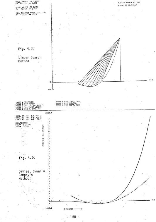
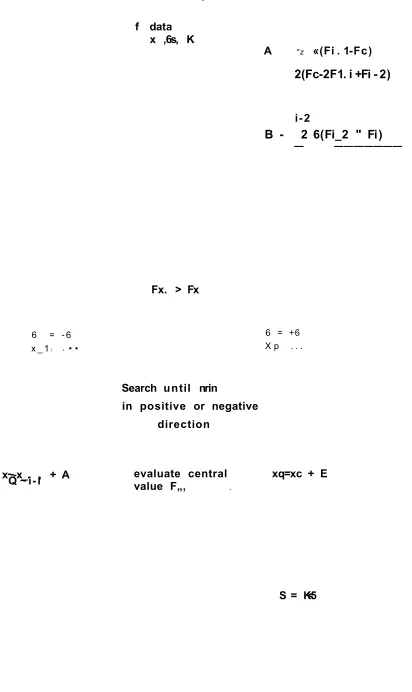
Davies, Swann and Campey's (19) method involves taking steps of increasing size from the given starting point until the function values at each step indicate that the minimum has been overshot. An additional function evaluation at the centre of the final interval produces four equally spaced points which span the minimum. One of these points is redundant for the purpose of quadratic approximation. Therefore the point most remote from the evaluation giving a minimum value of the function is discarded. A single quadratic f i t through the final three test points is then used to interpolate the minimum. The process is repeated until the desired degree of accuracy has been reached.
Powell's algorithm (20) differs from that of Davies, Swann and Campey in that a step of fixed length is taken from the given in itia l point, giving a second point. From the values of the function at these two points a third point is calculated. The minimum of a quadratic f i t through these three points is
then located and the test point which yields the highest functions value is rejected. The two remaining test points and the point of minimum given by the quadratic f i t are then taken to be the updated three points for a further quadratic f it . The process is repeated until the required minimum has been reached to within the desired accuracy.
Less efficient, but often used on account of their simpli city are the 'direct search' univariate methods such as
Fribonacci (21) and Golden section (22) algorithms. (b) Gradient Methods
There are two types of gradient methods. Methods which require the firs t derivatives of the objective function only, and those methods which need the firs t and second derivatives of the objective function in order to obtain the optimum.
The three methods of the firs t category which are investi gated later in this thesis are,
(1) Midpoint method (2) Linear search method (3) Davidson's method
The midpoint and linear search methods find the derivative of the objective function, and evaluate i t at the two points defining the search region. The value of the derivatives at a third point is then calculated. This point replaces one of the other two points, depending on the sign of the derivative value when compared with the value of the other two derivatives.
As for the non-gradient methods, Davidson's method predicts the location of the minimum through repeated use of a low order polynomial f i t (cubic) through the test points. This method is
-very powerful, but is limited to functions with fin ite and continuous firs t and second derivatives.
The second type of gradient method consists of those
which require explicitly the second derivatives of the objective function. One of the methods in this category is the Newton-Raphson method.
Some of the methods for one-dimensional objective functions mentioned‘so far have been extended to the multi-dimensional case where a sequence of one-dimensional searches is carried out in the multi-dimensional space along multi-dimensional search directions.
2.5.2.2 Methods for Multi-dimensional Objective Function
In the previous section the problem of finding the optimum value of a function with one variable was considered. It was found that the various types of methods were each most suitable for differing classes of functions, and situations. The same conclusion can be expected to hold when the number of variables is increased.
In general the optimization methods to solve multi-dimensional functions can be classified into two broad categories:
(i) Gradient methods ( ii) Direct search methods.
(i) Gradient Methods
The gradient methods can be divided into two groups, depending on whether they require matrix inversion or not.
(a) Methods with matrix inversion
The two methods included in this category are the Newton-Raphson method (23), and its variations, and Powell's algorithm
(24) specifically for minimizing a sum of squared terms.
-The Newton-Raphson method requires the exact determina tion of the inverse of the second derivative matrix, G. The iterative form is
-1
x(k+l) “ xk ' (k) 9(k) 5
where g is the -1 gradient vector. This method does not reach an optimum i f the second derivative matrix is not positive
definite. This also causes the method not to distinguish between
maxima, minima and saddle points.
Many variations of Newton-Raphson have been proposed, and the most common ones are the Quasi-Newton or variate metric formulae. These were f ir s t proposed by Davidon in 1959 and were
based on the fact that for a quadratic function y = G d for all k,
Wher% „ g( W ) . g{k) ,
(2.D
and d = >:( W ) . XW
Given a positive definite matrix H^0 *, the basic idea is to construct a sequence of matrices having the property
that
by imposing the quasi-Newton conditions
H<k+1) y - d (2. 2)
Biggs and Dixon (25) suggested an algorithm in which the
Newton-Raphson prediction is made whenever i t is possible to do so, but a step in the direction of the gradient is substituted for i t where G is singular.
-Powell's algorithm has proved to be efficient on a large range of functions. With this method the number of function evalautions required is usually for less than with methods which do not explicitly recognise the sum of squared terms, and also there is a reduction in computing from a third order to second order arithmetic step per iteration. An improved version of this method due to Powell (26) is available, which retains the
advantages described above, and it also improves a constraint in the direction of steepest descent as the step length is decreased. It appears that for difficu lt test cases, this is one of the consistently successful algorithms in this category. However, as with all algorithms that involve the inversion of a matrix, its efficiency will fa ll as the number of variables increases.
(b) Methods without matrix inversion
One of the oldest of all numerical methods is Cauchy's steepest descent, which dates back to 1817. This method requires only a numerical approximation to the gradient, and the direction taken at each stage is that of the gradient. This method does ultimately converge, but the rate of convergence is rather poor.
Forsyth and Matzkin (27) advocate a procedure which j
involves steepest descent coupled with pattern move, known as the accelerated step descent search method. The advantages of this method are that it ,
(1) requires few iterations,
(2) does not require evaluation of the gradient at the start of each one dimensional search,
-(3) possesses the quadratic convergence property. In the region around their optima functions can be approximated by a quadratic function of the form
T T
F(X) = C + AX + 1 X GX (2.3)
where G is an n by n positive definite matrix, A is a column vector of coefficients, and C is a constant.
A set of column vectors U-j, ... Un can be defined
that are mutually conjugate with respect to ci, i.e .
ul
* Gu.
J = 0 for i j .Optimization methods based upon such vectors as sets of conjugate directions search, each direction in turn in search of the minimum. For a quadratic function of N variables, the optimum value of the function is expected to be found within N unidirectional searches. One such method which has been con-sidered in this thesis is that of Fletcher-Reeves (28). In this method a linear search is undertaken along each conjugate search direction using cubic interpolation. This method is described in more detail in chapter five.
( ii) Direct Search Methods
In many problems, the function value is d iffic u lt to
* evaluate, and the expression for the gradient may be complicated or even unavailable. In both cases i t is acceptable in principle to estimate the value of the gradient by numerical approximation methods and then apply one of the gradient methods. The calcu lation of these estimates may involve considerabel computation, and difficulties often arise when numerical rounding errors affect the estimate of the gradient and interact with the
-vergence criteria. Therefore, algorithms have been written that do not involve the gradient either accurately or approxi mately. These algorithms can be divided into three main
categories:
(a) Univariate search methods (b) Unidirectional search methods
(c) Methods based upon evolutionary operations.
(a) Univariate search methods
These methods search along predetermined directions. Two of the more commonly used algorithms in this category are those suggested by Hooke and Jeeves (29) and Rosenbrock (30).
The Hooke and Jeeves method is applicable to any continuous objective function. It combines univariate search with pattern moves. The basic pattern move takes incremental steps after suitable directions have been found by univariate search. If the search progresses well in terms of decrementing the objective function, the step size is then increased, otherwise the step size is decreased. When the step size is reduced below a set value the search is terminated.
The Rosenbrock algorithm is similar to the Hooke and Jeeves method in following a 'valley', but i t requires the re-orienta tion of the orthogonal direction to do so. The re-orientation of direction vectors is achieved by using the G ram Schmidt procedure. This algorithm does not depend on the properties of quadratic functions, and i t usually obtains a local optimum. However, for functions which are quadratic near their optimum this method is not efficient when compared with other methods which take the quadratic convergence property into consideration.
-(b) Unidirectional search methods
There are two variants of the unidirectional search approach, namely that of Davies, Swann and Campey and further methods based on conjugate directions.
The Davies, Swann and Campey method can be considered as a development of Rosenbrock's proposal of rotating the search directions. The final stage of linear search consists of a quadratic interpolation which couM equally be replaced by that of Powell. This method is restricted; to functions with finite and continuous firs t partial derivatives, because of the quad ratic interpolation used during the liinear searches.
The methods of conjugate search direction use a sequence of one-dimensional searches along conjugate search directions and have the advantage of being quadratically convergent.
One of the firs t methods to Be- based on conjugate search directions is due to Smith (31). Bt has the disadvantage of being rather inefficient for problems involving a large number of variables. There are two reasors; for this inefficiency. First, the method is unable to contlfnually update the test point
so that the optimum can be found the required degree of
accuracy for a non-quadratic objective function. Second, the firs t of the N search directions is explored N times more fre quently than the Nth search direction.
Powell's method (32) is an inprovement on Smith's method and uses a different approach for pnerating the conjugate directions. This method may fa il tta> produce an optimum for functions which have a steep valley skewed to the co-ordinate
-directions. This may be due to either loss of the quadratic convergence property, or by failure to generate new conjugate directions.
(c) Evolutionary operation methods
The original idea of evolutionary operation for optimiza tion was introduced by Box (33) for a large scale industrial operation using statistical methods. Although the method demands only continuity of the objective function, i t has the disadvan tage that a large number of function evaluations are required.
I f N is the number of independent variables of the objective
function, then the method requires function evaluations.
The use of a simplex in a 'h ill climbing1 context was f ir s t suggested by Spendleyand Hext (34). The number of vertices used in the simplex method is (N+l) of which N points are re-used in the next iteration. Hence, only one function evaluation is required for each iteration. The original simplex method of Spendly and Hext had d iffic u lty in negotiating a narrow curved valley and once out of the valley the simplex method could not expand for a quick move towards the extremum point. The method was further improved by Nelder and Mead (35) through the use of reflection, expansion and contraction coefficients. The main advantages of this method are; f ir s t , i t does not involve uni directional searches, and second, i t does not use quadratic approximations to the function, so i t can therefore be applied to functions that contain discontinuous derivatives and to func tions where the neighbourhood of the optimum may not be quadratic.