http://dx.doi.org/10.4236/jemaa.2014.61002
Monte Carlo Computer Simulation of Nonuniform Field
Emission Current Density for a Carbon Fiber
P. A. Golovinski1,2, A. A. Drobyshev1
1
Voronezh State University of Architecture and Civil Engineering, Voronezh, Russia; 2Moscow Institute of Physics and Technology (State University) (MIPT (SU)), Moscow, Russia.
Email: [email protected]
Received October 30th, 2013; revised November 29th, 2013; accepted December 21st, 2013
Copyright © 2014 P. A. Golovinski A. A. Drobyshev. This is an open access article distributed under the Creative Commons Attri- bution License, which permits unrestricted use, distribution, and reproduction in any medium, provided the original work is properly cited. In accordance of the Creative Commons Attribution License all Copyrights © 2014 are reserved for SCIRP and the owner of the intellectual property P. A. Golovinski A. A. Drobyshev. All Copyright © 2014 are guarded by law and by SCIRP as a guardian.
ABSTRACT
The field emission current from a carbon fiber is considered. As a model of emission of an elementary carbon tube, tunnel ionization of an electron from a short-range potential is taken. The exact solution for the wave func- tion in such a model allows obtaining an asymptotic expression for electron current. A computer model of trans- verse distribution of emission current of a carbon fiber is built on the basis of the Monte Carlo method that al- lows taking into account the random character of distribution of local emitter sources and the distribution of gains of an electric field in carbon nanotubes.
KEYWORDS
Field Emission; Carbon Fiber; Current Density; Short-Range Potential; Monte Carlo Method
1. Introduction
Carbon nanotubes (CNT) can be grown in the form of small sharp spikes capable of withstanding considerable electric current densities. This assumes high potentialities of application of CNT as field emission cathodes in high- power vacuum devices. Such devices with field emission cathodes seem to be ideal for space applications [1] in- cluding disinfection means. New electrical, mechanical, and thermal properties of CNT have attractive characte- ristics for producing stable currents of high density with relatively low electric fields. The comparative analysis of different properties of field emission cathodes is given in [2], and the review of technological features of manu- facturing emitters based on nanotubes is in [3], where it is noted also that, besides application in high-power visi- ble and near-UV light sources, field emitters based on CNT are promising for X-ray minilamps, electron mi- croscopy, and microdiodes.
The emission properties of an individual nanotube are described on the basis of the Fowler-Nordheim model [4,5] based on the phenomenon of quantum-mechanical tunneling of an electron under a barrier under the action
of a constant electric field. The current density in such a model is determined by the dependence j=AF2
(
3 2)
exp −bφ F φ, where F is the electric field strength,
φ is the electron work function, b=6.83 eV V nm ,⋅
2
1.541 mA eV V
A= ⋅ ⋅ − [6]. It should be noted that this formula was initially obtained for metal emitters, and its application to nanotubes requires introduction of certain corrections. More exact formulas for field emission cur- rent take into account an additional polarization potential [7].
tubes of the order of height of individual CNT.
Investigations carried out earlier showed that emitter nonuniformities influenced the current density, but they did not give an answer to the question about the trans- verse nonuniformity of the current itself in its propaga- tion from the cathode to the anode. At the same time, this nonuniformity directly affects also the nonuniformity of secondary radiation caused by the emission current in a target. To solve this problem, we will consider a model based on taking into account the contribution of elec- tronic amplitudes to the expression for the total current in case of three-dimensional tunnel ionization of different ways arranging point sources.
2. Mathematical Model of Short-Range
Potential
To describe the propagation of an electron wave in a constant uniform electric field, we will choose a model, in which each individual nanotube is a point source of electron waves. Let us consider a point source, in which an electron is bound by a short-range potential [10]:
( )
2π( )
V r r
r δ κ ∂ = − ∂
r (1) at the energy E= −2κ2 2m. The Schrödinger steady- state equation describing the decay of a quasi-stationary state in the constant uniform electric field with the strength F looks like
( )
( )
( )
2
2 2π
2
i
E F e x r
m ϕ κ δ r ϕ
+ ∇ + = ∂
∂
r r r
(2)
The solution of the Equation (2) is expressed in terms of the Green function GE
( )
r r,1 of the Schrödingersteady-state equation for an electron in a uniform elec- tric field [11,12]:
(
1)
2{
( ) ( )
( ) ( )
}
1, Ci Ai Ci Ai 2
E
m
G = a+ ′ a− − ′ a+ a−
− r r r r (3)
(
)
(
)
2 31 1 2
2
m
a F e x x E
F e
±
= − + ± − +
r r
The function Ci
( )
s is expressed in terms of the ordi- nary Airy functions Ai( )
s and Bi( )
s [13]: Ci( )
s =( )
( )
Bi s +iAi s . The OX axis is directed oppositely to the direction of the electric field F . The equation for
( )
,1 EG r r looks like the Equation (2) with substitution of the point nonuniformity δ
(
r−r1)
for the right side.At F=0 the solution of the Equation (2) is
( )
(
)
0 exp 2π r r r κ κϕ = − (4)
The Equation (2) can be written as the equivalent integral equation
( )
3( ) ( )
( )
1 1 1 1 1
1
2π
d r GE , r
r
ϕ δ ϕ
κ ∂ = ∂
∫
r r r r r (5)
In the three-dimensional δ-potential [14] in the limit of a weak field the polarizability of a level is α=1 4κ4, and its width is
2 3
2 exp
2 3
e F
m e F κ κ
Γ = −
(6)
Substituting the undisturbed wave function (4) in the right side of the Equation (5), we will obtain
( )
2πGE( )
, 0 ,ϕ r = − κ r (7) and the current density at a great distance from the source is proportional to the squared absolute value of the wave function:
( )
2( )
2~ ~ E , 0
j ϕ r G r (8) For convenience of calculations it is advisable to write the solution in the asymptotic form:
( )
(
(
)
)
(
)
(
)
3 2
3 2
~ exp 2
3
exp 2
3
m
F e r x E F e
i m
F e r x E F e
ϕ − − −
× + + r (9)
At great distances from the source in the paraxial re- gion 2 2 r x x ρ − ≈ , 2 2 2
r x x
x ρ
+ ≈ + , where ρ= y2+z2 is the distance from the OX axis. Using the condition
2
4
F e E Fx e
x ρ
, we will obtain in the paraxial region:
( )
3 2 23 2 2 exp 2 3 4 exp exp 3 4 i
mF e x
x
m m
F e x
ρ ϕ κ κρ ≈ + × − × − r (10)
As a result, for the current from one point source we have the transverse distribution
3 2
~ exp exp
3 4
m m
j
F e x
κ κρ − × −
(11)
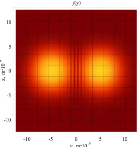
Shown in Figure 1 is the transverse distribution of electron current calculated by the formula (8) with the true Green function and by the asymptotic formula (11).
Figure 1. The transverse current distribution for the distance x=50 nm and the electric field strength F =
13
5 10 V m× : exact solution is solid curve, asymptotic re-presentation is dotted curve. The electron binding energy is
E =5 eV.
At longer distances the accuracy becomes still higher. So for practical calculations it is advisable to use just asymptotic expressions.
For several coherent centers the current density is
( )
2 32 2 2
2
~ ~ exp
3 2
exp exp
4 4
k k
k k
k k k
m j
F e
mF e m
i
x x
κ ϕ
κρ ρ
−
× × −
∑
∑
r
(12)
[image:3.595.311.536.84.322.2]where summation is made over all coherent sources.
Figure 2 shows the result of calculation of superposi- tion of coherent electron waves from two point sources. The distance to the screen and the binding energy cor- respond to Figure 1. The distance between the sources is
10 nm
R= .
In Figure 2 it is well seen that in the region of over- lapping of coherent waves interference shows itself.
3. Results of Computer Simulation
The statistical treatment of the values of the work func- tion for nanotubes gives an average value of the work function of 5.3 eV. It does not differ greatly from a cor- responding value for graphite. In this case a usual elec- tron energy spread is 0.3 eV. Moreover, if the source of field emission electrons is a carbon fiber, the emitter surface is very nonuniform and consists of randomly oriented carbon nanotubes, or has a flaky fibrillar struc- ture [15]. A characteristic number of fibrils in an emitter with an end area of 4 10× −7cm2 is up to 4000 elements. Accordingly, for each nanotube there is its own field gain
β that obeys the normal distribution law
Figure 2. The structure of interference fringes in interfe- rence of two coherent electron waves.
( )
(
0)
22
1 exp π
P β β β
β β
−
= −
∆
∆ (13)
The value typical of experiment treatment is ∆β β =
1.1 0.3÷ , and gains themselves vary in the rangeβ ~
2 4
10 ÷10 [8]. Such a spatial nonuniformity as well as strong temporal current fluctuations [16] exclude inter- ference effects, and the current density becomes the sum of currents of individual sources of the ensemble:
2 3
2
~ exp exp
3 2
k k
k k k k
m m
j j
F e x
κρ κ
β
= − −
∑
∑
(14)The nonuniformity of distribution of field gain over the emitter surface is confirmed by the results of direct measurement with the use of a scanning anode tunnel emission microscope [5]. At the same time, observed in this work was the distribution of field emission current density for a carbon emitter by luminescence on a lumi- nescent screen. As the field changed from F=2.5 Vµm
to F=3.1 V µm, on the 1.1 cm × 0.7 cm screen a sharp
increase of the total exposure field and increasing lumi- nescence uniformity were observed. The planar emitter sample under study had 164 point emitters located on an area of 2.4 10× −5cm2, that is, with a surface density of point sources of 6.8 10 cm× 6 −2.
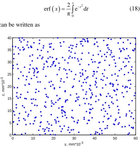
[image:3.595.65.286.380.455.2]Figure 3. The minimum distance between individual sources is limited by the parameter d=0.5 mµ that makes it possible to avoid superposition of sources, that is, to take into account the excluded volume effect.
In this case it is necessary, besides coordinates, to spe- cify the field gain βk for each source that is chosen
according to the random distribution (13).
An ordinary random number generator gives a uniform distribution in the interval (0,1). For an arbitrary density of distribution P x
( )
the distribution function [18] is determined by the relation( )
( )
1 d1x
F x P x x
−∞
=
∫
(15)Since the density of distribution is P x
( )
≥0, the dis- tribution function is a monotonically increasing function of x from F( )
−∞ =0 to F( )
∞ =1. This gives the single-valued inverse function( )
1
x=F− y (16) if y=F x
( )
. If now we in a random manner generate numbers u in the interval (0,1) with a uniform density, they will be mapped into a required distribution by the function r=F−1( )
u [19].For the normal distribution (13)
( )
(
1 0)
21 2
1
exp d
π
F
β β β
β β
β β
−∞
−
= −
∆
∆
∫
(17)which in view of the determination of the error function [17]
( )
20
2 erf e d
π
x t
[image:4.595.59.288.468.706.2]x =
∫
− t (18) can be written asFigure 3. The random arrangement of sources with ex- cluded volume.
( )
1 0erf 1
2
F β β β
β − = +
∆
(19)
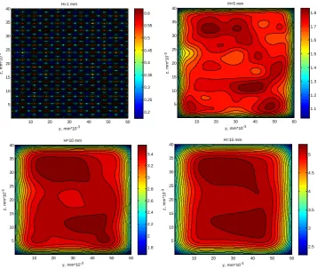
Shown in Figure 4 are the results of calculation of the distribution of current density F =2.5 10 V cm⋅ 7 ,
150
β= for different distances H between the emitter and the screen.
The results of calculations show high nonuniformity of transverse distribution of current density that decreases with growing number of point sources, field strength, and distance from the emitter to the screen. The ratio of the minimum current density to the average value jmin j
increases with distance from 0 to 0.5. The ratio of the maximum current density to the average value jmax j
decreases with growing distance to the screen from 4.6 to 3. In this case the spread of values estimated by the ratio of dispersion to the average value σj j remains high
at a level of 0.77 0.8÷ . This result should be assigned first of all to great fluctuations of density of arrangement of individual sources on the emitter surface.
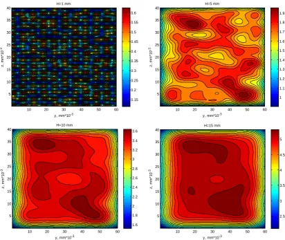
For comparison, shown in Figure 5 are the results of computer simulation in case of location of sources at points of a perfect square lattice at N=176 and with a step for lattice points of 4 µm. In this case the dimen- sions of regions with uniform current density are in- creased considerably, and low current densities are re- tained only on the edges of the screen. The ratio of the maximum density to the average value is jmax j = 1.8 2÷ , and the relative dispersion is σj j ~ 0.6. Thereby it was demonstrated that the regular arrange- ment of emission microsources increases significantly the current uniformity.
To find out the influence of partial disordering on the current structure, simulation was carried out with random shifts at a level of 20% distortion of a lattice constant. The results of simulation are presented in Figure 6. The comparison of calculations with the pattern obtained with regular arrangement of individual sources has shown that
max
j j increases no more than by 1%, and σj j
becomes only 0.3% more. Hence it follows that partial disordering of a regular structure retains general charac- teristics of degree of current nonuniformity.
4. Conclusions
The investigation carried out has shown that it is conve- nient to describe propagation of electrons from a field carbon emitter on the basis of exact Green functions of the Schrödinger equation in a uniform electric field. Each protruding element of the carbon fiber end surface can be simulated by a point source of electron waves. The high nonuniformity of sources results in loss of coherence for different sources and in nonuniform density of electron
0 10 20 30 40 50 60
0 5 10 15 20 25 30 35 40
y, mm*10-3
z
, mm*
1
0
[image:5.595.117.478.84.391.2]
Figure 4. The shadowgraph of distribution of current from random sources.
Figure 5. The shadowgraph of distribution of current from regularly arranged sources. y, mm*10-3
z
, mm*
1
0
-3
H=1 mm
10 20 30 40 50 60
5 10 15 20 25 30 35 40
0.5 1 1.5 2 2.5 3
y, mm*10-3
z
, mm*
1
0
-3
H=5 mm
10 20 30 40 50 60
5 10 15 20 25 30 35 40
1 2 3 4 5 6 7
y, mm*10-3
z
, mm*
1
0
-3
H=10 mm
10 20 30 40 50 60
5 10 15 20 25 30 35 40
1 2 3 4 5 6 7 8 9 10 11
y, mm*10-3
z
, mm*
1
0
-3
H=15 mm
10 20 30 40 50 60
5 10 15 20 25 30 35 40
2 4 6 8 10 12 14
y, mm*10-3
z
, mm*
1
0
-3
H=1 mm
10 20 30 40 50 60
5 10 15 20 25 30 35 40
0.2 0.25 0.3 0.35 0.4 0.45 0.5 0.55 0.6
y, mm*10-3
z
, mm*
1
0
-3
H=5 mm
10 20 30 40 50 60
5 10 15 20 25 30 35 40
1.1 1.2 1.3 1.4 1.5 1.6 1.7 1.8
y, mm*10-3
z
, mm*
1
0
-3
H=10 mm
10 20 30 40 50 60
5 10 15 20 25 30 35 40
1.8 2 2.2 2.4 2.6 2.8 3 3.2 3.4
y, mm*10-3
z
, mm*
1
0
-3
H=15 mm
10 20 30 40 50 60
5 10 15 20 25 30 35 40
[image:5.595.120.478.417.720.2][image:6.595.92.505.84.431.2]
Figure 6. The shadow graph of distribution of current from regularly arranged sources in case of random shifts in their ar- rangement.
current distribution, and in calculations of field emission it is possible to sum densities of currents from individual sources.
Simulation by the Monte Carlo method allows obtain- ing characteristic patterns of current distribution for dif- ferent densities of sources, field gains, and distances to the screen. Going from the random distribution of sources to their regular arrangement, even in case of partial loss of the order, considerably increases the current unifor- mity. The developed model allows choosing preferable parameters to increase the efficiency and life of radiation sources based on field carbon emitters.
Acknowledgements
The work has been done with the financial support of Russian Foundation for Basic Research (grant 13-07- 00270) and RF Government Contract No. 14.513.11.0133.
Conflict of Interest
The authors declare that there is no conflict of interests regarding the publication of this article.
REFERENCES
[1] P. Verma, S. Gautam, S. Pal, et al., “Carbon Nanotube- Based Cold Cathode for High Power Microwave Vacuum Electronic Devices: A Potential Field Emitter,” Defence Science Journal, Vol. 58, No. 5, 2008, pp. 650-654. [2] Y. Cheng and O. Zhou, “Electron Field Emission from
Carbon Nanotubes,” Comptes Rendus Physique, Vol. 4, No. 9, 2003, pp. 1021-1033.
http://dx.doi.org/10.1016/S1631-0705(03)00103-8
[3] H. S. Kim, D. Q. Duy, J. H. Kim, et al., “Field Emission Electron Source Using Carbon Nanotubes for X-Ray Tubes,”
Journal of the Korean Physical Society, Vol. 52, 2008, pp. 1057-1060. http://dx.doi.org/10.3938/jkps.52.1057
[4] R. H. Fowler and L. Nordheim, “Electron Emission in In- tense Electric Fields,” Proceedings of the Royal Society A, Vol. 119, 1928, pp. 173-181.
http://dx.doi.org/10.1098/rspa.1928.0091
[5] P. Gröning, P. Ruffieux, L. Schlapbach, et al., “Carbon Nanotubes for Cold Electron Sources,” Advanced Engi- neering Materials, Vol. 5, No. 8, 2003, pp. 541-550. http://dx.doi.org/10.1002/adem.200310098
[6] S.-D. Liang and L. Chen, “Generalized Fowler-Northeim Theory of Field Emission of Carbon Nanotubes,” Physi-
y, mm*10-3
z
, mm*
1
0
-3
H=1 mm
10 20 30 40 50 60
5 10 15 20 25 30 35 40
0.15 0.2 0.25 0.3 0.35 0.4 0.45 0.5 0.55 0.6
y, mm*10-3
z
, mm*
1
0
-3
H=5 mm
10 20 30 40 50 60
5 10 15 20 25 30 35 40
1 1.1 1.2 1.3 1.4 1.5 1.6 1.7 1.8 1.9
y, mm*10-3
z
, mm*
1
0
-3
H=10 mm
10 20 30 40 50 60
5 10 15 20 25 30 35 40
1.6 1.8 2 2.2 2.4 2.6 2.8 3 3.2 3.4 3.6
y, mm*10-3
z
, mm*
1
0
-3
H=15 mm
10 20 30 40 50 60
5 10 15 20 25 30 35 40
cal Review Letters, Vol. 101, Vol. 4, 2008, Article ID: 027602.
[7] Ch. Adessi and M. Devel, “Theoretical Study of Field Emission by Single-Wall Curbon Nanonotubes,” Physical Review B, Vol. 62, No. 20, 2000, pp. R13314-13317. http://dx.doi.org/10.1103/PhysRevB.62.R13314
[8] A. B. Elitskii, “Carbon Nanotube-Based Electron Field Emitters,” Physics-Uspekhi, Vol. 53, No. 9, 2010, pp. 863-892.
http://dx.doi.org/10.3367/UFNe.0180.201009a.0897
[9] G. B. Bocharov and A. V. Eletskii, “Theory of Carbon Nanotube (CNT)-Based Electron Field Emitters,” Nano- materials, Vol. 3, 2013, pp. 393-442.
http://dx.doi.org/10.3390/nano3030393
[10] Yu. N. Demkov and V. N. Ostrovsky, “Zero-Range Po- tentials and Their Application in Atomic Physics,” Ple- num Press, New York, 1988.
[11] B. Gottlieb, M. Kleber and J. Krause, “Tunneling from a 3-Dimensional Quantum Well in an Electric Field: An Analytic Solution,” Zeitschrift für Physik A Hadrons and Nuclei, Vol. 339, No. 1, 1991, pp. 201-206.
http://dx.doi.org/10.1007/BF01282950
[12] D. Gottlieb and M. Kleber, “Tunneling Dynamics in Sta- tionary Field Emission,” Annalen der Physik, Vol. 504,
No. 5, 1992, pp. 369-379.
http://dx.doi.org/10.1002/andp.19925040507
[13] M. Abramowitz and I. A. Stegun, “Handbook of Mathe- matical Functions,” National Bureau of Standards, Wa- shington DC, 1972.
[14] Yu. N. Demkov and G. F. Drukarev, “Decay and the Po- larizability of the Negative Ion in an Electric Field,” So-viet Physics JETP, Vol. 20, 1965, pp. 614-618.
[15] B. V. Bondarenko, Yu. L. Rybakov and E. P. Sheshin, “Field Emission of Carbon Fiber,” RE No. 8, Vol. 1593, 1982 (in Russian).
[16] E. P. Sheshin, “The Surface Structure and Field Emission Properties of Carbon Materials,” MIPT, Moscow, 2001.
[17] K. Cahill, “Physical Mathematics,” Cambridge University Press, Cambridge, 2013.
http://dx.doi.org/10.1017/CBO9780511793738
[18] W. Feller, “An Introduction to Probability Theory and Its Applications,” Vol. 1, Wiley & Sons, New York, 1968.