Munich Personal RePEc Archive
Understanding Interstate Trade Patterns
Yilmazkuday, Hakan
June 2009
Understanding Interstate Trade Patterns
Hakan Yilmazkuday
yJune 2009
Abstract
This paper models interstate trade patterns of U.S. states using a partial equilibrium trade model. The theoretical model deviates from the existing gravity literature by employing trade estimations in ratio form, with the ratio of imports from di¤erent sources, rather than the level of bilateral trade between two locations. Using this speci…cation, together with considering the production side through technology levels, the elasticity of substitution across goods, the elasticity of substitution across varieties of each good, and the good speci…c elasticity of distance measures are all identi…ed in the empirical analysis, which is not the case in gravity type studies. The ratio transformation also e¤ectively eliminates any proportional distribution margin, international trade, or overstatement of distance measures from the theoretical trade equation. Compared to empirical inter-national trade literature, the elasticity of substitution is estimated to be lower, while the elasticity of distance is estimated to be higher intranationally.
JEL Classi…cation: R12, R13, R32
Key Words: Trade Ratios; Transportation; The United States
1. Introduction
What is the main motivation behind intranational trade? Compared torelatively complex models in the literature, this paper contributes by introducing a simple partial equilibrium model to analyze the motivations behind bilateral trade patterns of regions at thedisaggregate level. It is attempted to …nd why regions do import more goods from some regions while importing fewer from others. It is also investigated why a region imports more of a good while importing less of another one. A monopolistic competition model consisting of a …nite number of regions is employed. There are two types of goods, traded and nontraded. Each region produces and consumes a unique nontraded good. Each region may also consume all varieties of all traded goods, while it can produce only one variety of each traded good. While the traded goods are produced by a perfectly mobile unique factor, the only nontraded good in each region is produced by the same mobile factor together with traded intermediate inputs. According to this setup, as is standard in the literature, it is shown that the trade of a variety of a particular traded good across any two regions depend on the relative price of the variety and the total demand (…nal consumption demand plus intermediate input demand) of the good in the destination (importer) region. The nuance of this paper comes into the picture when the ratio between imports of varieties from di¤erent sources (exporters) is considered. It is found that a region imports more goods (measured in values) from the lower price regions and fewer goods from the more distant regions.
Considering the ratio between imports of varieties from di¤erent sources (rather than the level of bilateral trade between two locations) has several empirical and analytical bene…ts compared to gravity models in the following senses:
(i) There is no identi…cation problem in terms of estimating the elasticity of substitution and the elasticity of distance at the same time. However, even Anderson and van Wincoop’s (2003) most popular gravity model su¤ers from this problem (also see Wei 1996; Hummels 1999, 2001). By distinguishing between aggregate level and disaggregate level trade data, together with considering the production side of the model, the elasticity of substitution across goods can also be estimated. The main idea is to exploit (implicit) variation in prices (which
I thank Eric Bond, Mario Crucini, Kevin Huang, David Hummels, Meredith Crowley, Brown Bag Seminar participants at Vanderbilt University, Midwest International Economics Meeting participants in University of Illinois at Urbana-Champaign, SRSA Annual Meeting participants in Arlington, VA-Washington, DC for their helpful comments and suggestions. All errors are my own responsibility.
yDepartment of Economics, Temple University, Philadelphia, PA 19122, USA; Tel: +1-215-204-8880; Fax: +1-215-204-8173; e-mail:
can be proxied by variation in inferred technology parameters that are imputed from data on production and cost of living data) across origins to pin down the elasticity of substitution across varieties. Having pinned down the elasticity of substitution across varieties, independently of distance, one can identify the elasticity of distance directly o¤ the estimated distance coe¢cient.
(ii) The methodology controls for a possible issue of overstating the distance measures (due to using calculated distances, such as great circle distances) mentioned by Hillberry and Hummels (2001), given the overstatement is proportional to the actual distance measures.
(iii) By construction, the model is capable of controlling for the proportional e¤ects of local (i.e., wholesale and retail) distribution costs, insurance costs, local taxes, markup di¤erences in production, international trade (under reasonable assumptions), and intermediate input trade, each of which are possible topics for separate debates in the literature (see Anderson and van Wincoop 2004).
(iv) There is an exogenous solution for the estimated trade expression, and thus, there is no need for any income data for estimation,given the technological levels. This convenient feature of the model also makes the estimation free of a possible endogeneity problem.
The model is estimated using bilateral trade data belonging to the states of the U.S. The estimated parameters correspond to: a) elasticity of substitution across varieties of a good, each produced in a di¤erent region; b) elasticity of substitution across goods, each consisting of di¤erent varieties; c) elasticity of distance, which governs good speci…c trade costs; and d) heterogeneity of individual tastes, governing geographic barriers and the so-called home-bias. Several strategies are pursued to estimate these parameters and the results are supported with di¤erent sensitivity analyses. Overall, the model is capable of explaining the interstate trade data up to 84% at the disaggregate level, and up to 77% at the aggregate level.
The estimated parameters give insights about a number of issues related to interstate trade patterns within the U.S.: a) compared to empirical international studies, elasticity of substitution is lower intranationally; b) compared to empirical international studies, elasticity of distance is higher intranationally; c) there is evidence of home-bias even at the intranational level; d) trade costs are mostly good speci…c even at the intranational level; e) source-speci…c …xed e¤ects are important for bilateral trade patterns, e¤ects usually ignored in the literature; f) production technologies are both good and region speci…c rather than country speci…c; g) elasticity of substitution across varieties is good speci…c.
Related Literature
This subsection describes how this paper relates to its closest antecedents, especially gravity type studies. The gravity models are popular mostly due to their empirical success.1 When the theoretical background of gravity
type studies is considered, Anderson (1979) is the …rst one to model gravity equations. The main motivation behind Anderson’s (1979) gravity model is the assumption that each region is specialized in the production of only one good.2 Despite its empirical success, as Anderson and van Wincoop (2003) point out, the specialization assumption suppresses …ner classi…cations of goods, and thus makes the model useless in explaining the trade data at the disaggregate level. Another de…ciency of Anderson’s (1979) gravity model is the lack of a production side. Bergstrand (1985) bridges this gap by introducing a one-factor, one-industry,N-country general equilibrium model in which the production side is considered. In his following study, Bergstrand (1989) extends his earlier gravity model to a two-factor, two-industry,N-country gravity model.3
The main de…ciency of the gravity models is that they cannot control for good speci…c transportation costs, good speci…c local (i.e., wholesale and retail) distribution costs, good speci…c insurance costs, good speci…c local taxes, region speci…c markup di¤erences in production, good speci…c intermediate input trade or international trade. Moreover, one cannot estimate the elasticity of substitution and the elasticity of distance at the same time using gravity equations. However, this paper controls for all of these situations.
None of the papers mentioned above empirically deal with the trade patterns within a country. Recently, Wolf (2000), Hillberry and Hummels (2001), and Millimet and Thomas (2007) bridged this gap by analyzing the interstate trade patterns within the U.S. However, these studies have a de…ciency, because they use the aggregate level (i.e., total bilateral) trade data, while this paper uses disaggregate level bilateral data that give more insight related to good speci…c analyses. Another de…ciency of these studies is that they use gravity type models which su¤er from the same issues mentioned above. Also, these studies cannot distinguish between the elasticity of substitution
1Deardor¤ (1984) reviews the earlier gravity literature. For recent applications, see Wei (1996), Jensen (2000), Rauch (1999),
Helpman (1987), Hummels and Levinsohn (1995), and Evenett and Keller (2002).
2In the Appendix of his paper, Anderson (1979) extends his basic model to a model in which multiple goods are produced in each
region.
3Also see Suga (2007) for a monopolistic-competition model of international trade with external economies of scale, Lopez et al.
across varieties of a good, elasticity of substitution across goods, and the elasticity of distance at the same. By taking the ratio between imports of varieties from di¤erent origins (exporters), by taking the ratio between imports of di¤erent goods, and by including intermediate input trade into the model, this paper takes care of all of these issues by construction.
Nevertheless, this paper is not the …rst one that considers trade ratios. For instance, studies such as Head and Ries (2001), Head and Mayer (2002), Eaton and Kortum (2002), and Romalis (2007), among others, have also considered trade ratios in their gravity type models. Most of these studies have attempted to eliminate price measures from the gravity equation since they see them as nuisances. In order to get rid of those price measures, one cannot simply take the ratio among imports of varieties from di¤erent origins; they also have to consider the ratio among imports of varieties within regions. This process results in having an index of freeness of trade that determine the impacts of borders (mostly related to international trade literature) rather than explaining the intranational trade patterns. Although this approach seems …ne up to a point, it has the de…ciency of not considering the production side at all and not having a structure to analyze the disaggregate level trade. The closest study to this paper is by Romalis (2007). However, by eliminating the source speci…c marginal costs (i.e., the production side), Romalis (2007) cannot identify the elasticity of substitution and the elasticity of distance at the same time; instead, he can only estimate the elasticity of substitution. By considering the production side, this paper can estimate the elasticity of substitution and the elasticity of distance at the same time. Moreover, all of these studies also don’t take into account zero trade observations that have a high share in overall observations.4 This paper contributes
to the literature by controlling for all of these issues, therefore by having accurate empirical results.
Plan of the Paper
The rest of the paper is organized as follows. Section 2 introduces a regional trade model. Section 3 introduces data. Section 4 provides insights and depicts the estimation methodology. Section 5 depicts empirical results, while Section 6 concludes.
2. The Model
An economy consisting of a …nite number of regions is modeled. In each region, there are two types of goods, traded and nontraded. While a unique nontraded good is produced and consumed within all regions (thus, the nontraded goods market is in equilibrium in each region separately), each region may consume all varieties of all traded goods and can produce only one variety of each traded good. Since the partial equilibrium bilateral trade implications of the model is su¢cient for an empirical analysis, in many instances, the irrelevant details of the model are skipped to keep the model more trackable.
Each traded good is denoted byj= 1; :::; J. Each variety is denoted byithat is also the notation for the region producing that variety. The analysis is made for a typical region, r. In the model, generally speaking, Ha;b(j)
stands for the variableH, whereais related to the region of consumption,bis related to the variety (and thus, the region of production), andj is related to the good.
2.1. Individuals
The representative agent in regionrmaximizes utilityU CT
r; CrN T whereCrT is a composite index of traded goods
andCN T
r is a unique nontraded good. The composite index of traded goods,CrT, is given by:
CrT
0
@X
j j
1
" CT
r (j)
" 1
"
1
A
" " 1
whereCT
r (j)is given by:
CrT(j) X
i
( r i) (1j) CT
r;i(j)
(j) 1 (j)
! (j) (j) 1
whereCT
r;i(j)is the varietyiof traded goodj imported from regioni;" >0 is the elasticity of substitution across
goods; (j) >1 is the elasticity of substitution across varieties of good j; j is a good speci…c taste parameter;
r is a destination (i.e., importer) speci…c taste parameter; and …nally, i is a source (i.e., exporter) speci…c taste
parameter. For di¤erent varieties, while having only one bilateral taste parameter, which is both destination and
source speci…c, is standard in the literature, decomposing it into r and i is new in this paper.5 In particular,
both r and i can be used as …xed e¤ects in a regression analysis; i.e., they together represent a unique bilateral
taste parameter between regionsrandi. Moreover, by putting restrictions on i, one can easily measure home-bias
implications of the model. Besides, one can also control for issues such as migration by using i (see Millimet and
Thomas, 2007). For robustness, the validity of this assumption is tested in Section 5.
The optimal allocation of any given expenditure within each variety of goods yields the following demand functions:
Cr;iT (j) = r i P
T r;i(j)
PT r (j)
! (j)
CrT(j) (2.1)
and
CrT(j) = j
PT r (j)
PT r
"
CrT (2.2)
wherePT r (j)
P
i r iPr;iT (j)
1 (j) 1 1(j)
is the price index of the traded goodj(which is composed of di¤erent
varieties), andPrT Pi jPrT(j)1 " 1 1 "
is the cost of living index in regionr. It is implied thatPrT(j)CrT(j) =
P
iPr;iT (j)Cr;iT (j).
2.2. Firms
Since there are two types of goods, namely traded and nontraded, there are two types of …rms in each region.
2.2.1. Production of Traded Goods
Traded goodj in regionr(i.e., variety rof goodj) is produced by the following production function:
YrT(j) =Ar(j)LTr (j) (2.3)
whereAr(j)represents the good and region speci…c technology, and LTr (j)represents a perfectly mobile factor of
production of which hour is worth W in all regions.6 The …rm chooses LT
r (j), taking as given its price W. The
cost minimization problem of the …rm implies that the marginal cost of producing varietyrof goodj (in regionr) is given by:
M CrT(j) =
W Ar(j)
(2.4)
Note that M CrT(j)is good and region speci…c.
Although having a perfectly mobile factor of production within the same country is a reasonable assumption, a conservative researcher may see it as a strong one; however, it has very convenient empirical implications. In particular, as it will be clearer below, when the ratio of imports from two alternative sources are considered, the price of this factor of production e¤ectively disappears. Nevertheless, the empirical analysis will still have the ratio of source speci…c technology levels, which captures the ratio of source speci…c wages up to some degree, because wages are highly correlated with productivity as is well known, especially, in the business cycle literature.7 In
particular, as will be introduced in data section below, when technology level for a particular good is calculated as the value added per labor hour divided by the cost of living index in each region, it is already assumed that real wages, rather than nominal wages, are equalized across regions, because labor responds to real wages, rather than nominal wages, in practice.
5Distinguishing between destination and source speci…c taste parameters has useful properties in terms of the estimation as shown
in Section 4.
6One can easily assumeL
r(j)to be labor and/or capital, but the results of this paper are not a¤ected at all by these details as we
will see below.
7In such a case, another problem may arise: if wages are highly correlated with technology levels, and if wages were region speci…c
2.2.2. Production of Nontraded Goods
The unique nontraded good in regionris produced by a production function YN T
r LN Tr ; GN Tr where LN Tr
repre-sents the completely mobile factor of production (i.e., the same factor used in the production of traded goods) and
GN T
r is the counterpart ofCrT given by:
GN Tr
0
@X
j j
1
" GN T
r (j)
" 1 " 1 A " " 1
whereGN T
r (j)is given by:8
GN Tr (j) X
i
( r i) (1j) GN T
r;i (j)
(j) 1 (j)
! (j) (j) 1
The optimal allocation of any given expenditure within each variety of intermediate inputs yields the following demand functions:
GN Tr;i (j) = r i
Pr;iT (j)
PT r (j)
! (j)
GN Tr (j) (2.5)
and
GN Tr (j) = j P
T r (j)
PT r
"
GN Tr (2.6)
Note that the …rms share the same taste parameters, r; i and j, with the individuals. Although this is a strong
assumption, it has very nice properties in terms of bilateral trade implications that are discussed in Section 4.
2.2.3. Trade Cost
Anderson and van Wincoop (2004) categorize the trade costs under two names, costs imposed by policy (tari¤s, quotas, etc.) and costs imposed by the environment (transportation, wholesale and retail distribution, insurance against various hazards, etc.). Since this paper considers trade within a country (i.e., the U.S.), the …rst category can be ignored, and focus is on the second one. Instead of assuming an iceberg transport cost, the transportation is achieved by a transportation sector, which is not modeled here.9 This assumption is important to distinguish
between the export income received by the exporter and the transportation income received by the transporter. The implications of this assumption will be clearer below. In particular, we assume that, if there is a trade between regions, it is subject to a transportation cost:10
Pi;rT (j) = (1 + i;r(j)) Pr;rT (j) (2.7)
= (Di;r) (j) Pr;rT (j)
wherePT
r;r(j)is the price of the traded good at the factory gate (i.e., the source); i;r(j)>0is a good speci…c net
transportation cost from regionrto regioni;Di;r is the distance between regionsrandi; and (j)is the elasticity
of distance.11;12 The cost implications of the model in terms of wholesale distribution, retail distribution, insurance
or local taxes, will be provided below.
8Since the bilateral trade implications of the model are su¢cient for the empirical analysis, after assuming that the nontraded goods
market is in equilibrium in each region, the exact functional forms of YN T
r LN Tr ; GN Tr , demand forLN Tr , and the marginal cost
implication for the nontraded goods are all irrelevant.
9Since the partial equilibrium bilateral trade implications of the model are su¢cient for the empirical analysis of this paper, the
actual role/model of the transportation sector is irrelevant after assuming that transportation is achieved by using the completely mobile factor of production (i.e., the same factor used in the production of traded/nontraded goods).
1 0Needless to say, the existence of trade is determined by Equation 2.1 for alli,randj. As we will discuss in detail in the following sections, we consider the absence of trade, besides the existence of it in our empirical analysis.
1 1For the distance within each state (i.e., the internal distance), we use the proxy developed by Wei (1996), which is one-fourth the
distance of a region’s capital from the nearest capital of another region.
1 2See Yilmazkuday (2008) for a theoretical model of transportation which connects(1 +
2.2.4. Equilibrium
Since the partial equilibrium bilateral trade implications of the model are su¢cient for an empirical analysis, the details for equilibrium in nontraded goods market are not depicted here; instead, equilibrium in the traded goods market is shown. In particular, for each variety r of traded good j produced in region r, the market clearing condition implies:
YrT(j) =X
i
Ci;rT (j) +X
i
GN Ti;r (j) (2.8)
where CT
i;r(j)is the demand of regioni for varietyrof traded good j (produced in regionr); andGN Ti;r (j)is the
intermediate input demand for variety rof traded good j (produced in region r) demanded for the production of the nontraded good in regioni . Equation 2.8 basically says that varietyrof …nal good j produced in regionr is either consumed locally or by other regions, either for …nal consumption or as an intermediate input.
2.2.5. Price Setting
Since the partial equilibrium bilateral trade implications of the model are su¢cient for an empirical analysis, the price setting behavior of the …rms producing the unique nontraded good in each region is skipped. For the traded goods, in regionr, a typical …rm that produces varietyrof traded goodj faces the following pro…t maximization problem:
max
PT r;r(j)
YrT(j) Pr;rT (j) M CrT(j)
subject to Equation 2.8 and the symmetric versions of Equation 2.1 and 2.5. The …rst order condition for this problem is as follows:13
YrT(j) 1 (j)
PT r;r(j)
Pr;rT (j) M CrT(j) = 0
which implies that:
Pr;rT (j) = (j)
(j) 1 M C
T
r (j) (2.9)
= (j) (j) 1
W Ar(j)
where (j() 1j) represents a good-speci…c (gross) mark-up.
2.3. Bilateral Trade
In order to depict all implications of the model, it is distinguished between disaggregate and aggregate level trade. While the disaggregate level trade considers bilateral ratios of imports of a region for di¤erent varieties of a particular good, the aggregate level trade considers bilateral ratios of imports of di¤erent goods for a particular region.
2.3.1. Disaggregate Level Trade
Using Equations 2.1, 2.5 and 2.7, an expression for the ratio of imports of regionrfrom source regionsaandb can be obtained as follows:
Xr;a(j)
Xr;b(j)
= a
b
Pb;bT (j)
PT a;a(j)
! (j) 1
Dr;b
Dr;a
(j) (j)
(2.10)
where Xr;k(j) = Cr;kT (j) +Gr;kN T(j) Pk;kT (j)is the value of total imports of regionr from regionk measured at
the source for goodj.14 Equation 2.10 says that a region imports more goods (measured in values) from lower price
regions and fewer goods from more distant regions.
1 3Notice that the …rm takes the composite consumption index of goodj(i.e., CT
r (j)), the composite index of intermediate demand
for good j(i.e., GN T
r (j)) and the composite price index of goodj (i.e.,PrT(j)) in each region as given in the optimization problem,
because the …rm is assumed to be too small to have an e¤ect on these variables.
1 4If we had an iceberg cost in our analysis, we would have hadX
r;k(j) = Cr;kT (j) +G N T r;k (j) P
T
k;k(j) 1 + r;k(j) as the export
income received by the exporter region for goodj. However, this is not the case in the real world that distinguishes between the exporter
Substituting Equation 2.9 into Equation 2.10 results in the general form of equations for the disaggregated level trade analysis:
Xr;a(j)
Xr;b(j)
= a
b
Aa(j)
Ab(j)
(j) 1
Dr;b
Dr;a
(j) (j)
(2.11)
Note that Equation 2.11 is an exogenous solution for the disaggregate level trade expression to be estimated, and thus, there is no need for any endogenous data, such as income, for the estimation, given the technology levels. Moreover, it can easily be estimated in log terms.
2.3.2. Aggregate Level Trade
Using Equations 2.2 and 2.6, an expression for the ratio of imports of regionr in terms of goods j and k can be obtained as follows:
Xr(j)
Xr(k)
= j
k
PT r (j)
PT r (k)
1 "
(2.12)
where Xr(m) = CrT(m) +GN Tr (m) PrT(m) =
P
i Cr;iT (m) +GN Tr;i (m) Pi;iT (j)D
(j)
r;i is the value of total
imports of regionr in terms of goodm measured at the destination.15 Equation 2.12 says that a region imports
more (less) of a good which has a lower (higher) destination price. Substituting Equations 2.7, 2.9, and PT
r (j)
P
i r iPr;iT (j)
1 (j) 1 1(j)
into Equation 2.12 results in the general form of equations to be estimated for the aggregate level trade analysis:
Xr(j)
Xr(k)
= j
k
0 B @
(j) (j) 1
P
i r iD
(j)
r;i (Ai(j)) (j) 1
1 1 (j)
(k) (k) 1
P
i r iD
(k)
r;i (Ai(k)) (k) 1
1 1 (k)
1 C A
1 "
(2.13)
Note that Equation 2.13 is an exogenous solution for the aggregate level trade expression, and thus, there is again no need for any endogenous data, such as income, for the estimation,giventhe technology levels. Moreover, it can easily be estimated in log terms after estimating the disaggregate level expression given by Equation 2.11 (i.e., after obtaining estimates for (j)’s and (j)’s).
3. Data
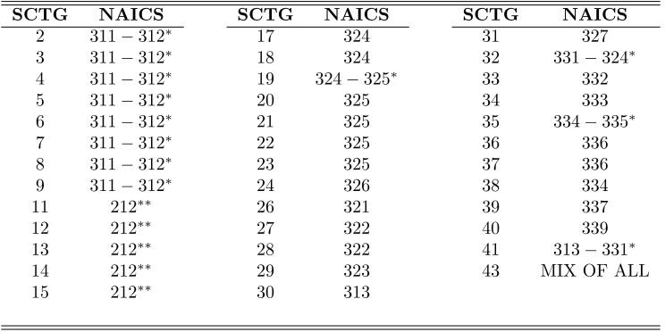
For the bilateral trade analysis, state-level Commodity Flow Survey (CFS) data obtained from the Bureau of Transportation Statistics for the United States for the year 2002 are used. CFS captures data on shipments originating from select types of business establishments located in all states of the U.S., however, because of data availability, Alaska, District of Columbia and Hawaii are excluded from the analysis. CFS depicts both source and destination states for the value of shipments (i.e., exports) that are measured at the source. This is a perfect match to test the model of this paper, especially through Equation 2.10. The disaggregated level exports data cover 2-digit Standard Classi…cation of Transported Goods (SCTG) commodities of which codes are given in Table 1. In this context, a typical sample from CFS data is the value of shipments of Alcoholic Beverages (of which SCTG code is 8) from New York to California. In CFS, shipments traversing the U.S. from a foreign location to another foreign location (e.g., from Canada to Mexico) are not included. Shipments that are shipped through a foreign territory with both the origin and destination in the U.S. are included in the CFS data.16 International export (import)
shipments are also included in CFS, with the domestic destination (source) de…ned as the U.S. port, airport, or border crossing of exit from the U.S.; e.g., an international export (import) of an Alcoholic Beverage entering to (exiting from) the U.S. through a port in New York is depicted as a shipment to (from) New York in CFS. This is an important feature of CFS that will be used in the empirical analysis below to control for international exports and imports.
In order to obtain good and region speci…c technology levels, an approximate mapping (that is o¢cially called a "crosswalk") between 3-digit North American Industry Classi…cation System (NAICS) and 2-digit SCTG obtained from the National Transportation Library of the Bureau of Transportation Statistics is employed. Using this
1 5Since the data set of Commodity Flow Survey includes only the export income received by the …rms, one has to distinguish between
the value of exports at the source and at the destination.
1 6The mileages calculated for these shipments exclude the international segments (e.g., shipments from New York to Michigan through
mapping given in Table 1,Ai(j) = PViLi(ij()j) is calculated for alli; j as a measure of technology, whereVi(j) is the
industry and state speci…c value added of the relevant NAICS industry obtained from U.S. Census Bureau in 2002,
Pi is the cost of living index for stateiborrowed from Berry et al. (2003) for the year 2002, andLi(j)is industry
and state speci…c hours of labor supplied by the production workers of the relevant NAICS industry obtained from U.S. Census Bureau in 2002.17 It is important to note that the level of technology already includes a measure of
wages through the cost of living index after assuming that real wages (rather than nominal wages) are equalized across regions. In other words, although the nominal wages are equalized across regions in the model to have more trackable framework, the real wages are equalized in the empirical analysis, because, as is standard in the literature, the labor respond to real wages rather than nominal wages in practice.
For distance measures, great circle distances between bilateral states are calculated. When calculating latitude and longitude of each state, the weighted average of latitudes and longitudes of the cities in that state are taken, where the weights are determined according to the production level of those cities. The production level in each city is measured by the real gross domestic product values obtained from Bureau of Economic Analysis (BEA) for 2002. By using these weights, more relevant spatial locations are obtained for measuring the potential interactions across states. Although an average distance measure is provided for eachobserved shipment in CFS, the benchmark analysis of this paper uses great circle distances, because the average distance measures in CFS are available only for realized trade observations. Since zero (trade) observations (i.e., the observation of no trade) are also considered in this paper, a more comprehensive distance measure is needed to capture the e¤ect of distance on the absence of trade. Nevertheless, for robustness, the estimation results obtained by great circle distances are compared with the results obtained by CFS distances in the sensitivity analysis #3 below.
4. Remarks and Estimation Methodology
A two-step estimation process is employed. First, the empirical power of the model is tested at the disaggregate level and estimates of elasticity of substitution across varieties of each good (i.e., (j)’s), and good speci…c distance elasticities (i.e., (j)’s) are obtained; these are used to obtain good speci…c price indices (i.e.,Pi(j)’s) according to
the model. Second, the empirical power of the model is tested at the aggregate level and the elasticity of substitution across goods (i.e.,") is estimated.
4.1. Disaggregate Level Trade Estimation
In this subsection, the implications of Equation 2.11 are provided, and di¤erent log versions of it that are used for robustness are introduced. Although Equation 2.11 holds on average, it doesn’t hold for each bilateral trade ratio. In empirical terms, following Santos Silva and Tenreyro (2006), and Henderson and Millimet (2008), to address the unobservable nature of bilateral trade ratios, it is assumed that there is an error term associated with each ratio, which implies that:
Xr;a(j)
Xr;b(j)
= a
b
Aa(j)
Ab(j)
(j) 1
Dr;b
Dr;a
(j) (j)
+ r;a;b;j
whereEh r;a;b;j a b;
Aa(j)
Ab(j);
Dr;b
Dr;a
i
= 0. This can be rewritten as:
Xr;a(j)
Xr;b(j)
= a
b
Aa(j)
Ab(j)
(j) 1
Dr;b
Dr;a
(j) (j)
r;a;b;j (4.1)
where
r;a;b;j= 1 + r;a;b;j
a b
Aa(j)
Ab(j)
(j) 1
Dr;b
Dr;a
(j) (j) (4.2)
andEh r;a;b;j ab;AAab((jj));
Dr;b
Dr;a
i
= 1. Taking the log of both sides in Equation 4.1 results in the following log-linear expression for the bilateral disaggregate level traderatios:
log Xr;a(j)
Xr;b(j)
= log a
b
+ ( (j) 1) log Aa(j)
Ab(j)
+ (j) (j) log Dr;b
Dr;a
+ log ( r;a;b;j) (4.3)
1 7Although value added is used for each industry to calculate technology levels, this should not be necessary the case in the presence of
a better measure of technology. In other words, the claim in the text saying "There is no need for any income datagiventhe technology
To obtain a consistent estimator of the slope parameters by the Ordinary Least Squares (OLS), it is assumed that
E
h
log ( r;a;b;j) ab;AAab((jj));DDr;br;a
i
does not depend on the regressors.18 Because of Equation 4.2, this condition is met
only if r;a;b;jcan be written as follows:
r;a;b;j= a b
Aa(j)
Ab(j)
(j) 1
Dr;b
Dr;a
(j) (j)
r;a;b;j
where r;a;b;jis a random variable statistically independent of the regressors. In such a case, r;a;b;j= 1+ r;a;b;jand
therefore is statistically independent of the regressors, implying thatEhlog ( r;a;b;j) ab;AAab((jj));DDr;ar;b
i
is a constant.
Following Santos Silva and Tenreyro (2006), the assumption of Ehlog ( r;a;b;j) ab;AAab((jj));
Dr;b
Dr;a
i
not depending on the regressors is relaxed in Sensitivity Analysis #4, below, by considering the Poisson Pseudo-Maximum Likelihood (PPML) estimator.
In the estimation,only one OLS (or PPML) regression is employed for the pooled sample by including relevant dummy variables for a
b; (j)and (j)in Equation 4.3. AlthoughAi(j)’s are region and good speci…c technology
levels in Equation 4.3, they don’t necessarily capture all the source speci…c …xed e¤ects. This is why source speci…c taste parameters (i.e., i’s) may play an important role in the estimation. For instance, in addition to the technology
levels, source speci…c …xed e¤ectsmay capture possible di¤erences in source speci…c production markups, source speci…c production taxes, and so on. The validity of having both these …xed e¤ects and technology levels at the same time are tested in Version B and Version G of the empirical estimation, below.19
According to Equation 4.3, the following remarks are implied:
Remark 1. Both (j)and (j)can be identi…ed in Equation 4.3 which is not the case in most gravity models (see Anderson and van Wincoop 2003; Hummels 1999, 2001; Wei 1996).
P roof. The identi…cation is realized via the technology levels which are usually ignored in gravity models. In particular, since both( (j) 1) and (j) (j)can be estimated by Equation 4.3, one can identify both (j)and
(j)while also calculating their standard errors by employing the Delta method.
Remark 2. All the variables in Equation 4.3 are exogenous, which leaves an applied researcher free from a possible endogeneity problem. Moreover, there is no need for income data given the exogenous technology levels.
P roof. The proof follows through Equation 2.11.20
Remark 3. Assuming that overstatement of a distance is proportional to the distance itself, the model controls for such an issue (because of the use of calculated distance measures such as great circle distances) as mentioned by Hillberry and Hummels (2001).
P roof. Assuming that overstatement of a distance is proportional to the distance itself, the distance ratio in Equation 4.3 is not a¤ected at all. See sensitivity analysis #3 in Section 5 for details.
Remark 4. By construction, the model is capable of controlling for the e¤ects of local (i.e., wholesale and retail) distribution costs, insurance costs or local taxes, each of which are possible topics for separate debates in the literature (see Anderson and van Wincoop 2004).
1 8It is well known that modeling zero interregional ‡ows using a normal error process leads to problems. If the dependent variable
cannot take a value below zero, then a normal error process is a poor approximation. Nevertheless, we don’t have such a concern, because our log-linearized equation does have values below zero, by considering the (log) ratio of bilateral trade values.
1 9Multicollinearity is less of a problem in a cross-sectional analysis like ours that has a high sample size. The reasoning is that we run
only one regression instead of good speci…c regressions; if we were running good speci…c regressions, then i’s andAi(j)’s would have
been perfectly correlated, because, in such a case, we would have good speci…c i’s. Moreover, the individual e¤ects of technology and
source speci…c taste parameters can both be assessed when there are su¢cient number of observations of high technology regions with low …xed e¤ects and low technology regions with high …xed e¤ects. Besides, the theoretical consequences of multicollinearity is still a debate, because even if the multicollinearity is very high, the OLS estimators still remain to be the best linear unbiased estimators. The only possible problem arises due to having wide con…dence intervals in the presence of multicollinearity. However, by having very low con…dence intervals, our estimation results below are robust to a possible multicollinearity problem. See Achen (1982) and Gujarati (1995) for more details.
2 0If trade leads to technology transfer, than technology may be correlated with past trade levels. And, if there are unobservables
P roof. To see this, consider Equation 2.1 by including such possible good speci…c proportional costs. For instance, say that there is a proportional (net) cost of'(j)for good j in regionr. Then, it follows that:
Cr;a(j) = a
Pr;a(j) (1 +'(j))
Pr(j) (1 +'(j))
(j)
Cr(j)
and
Cr;b(j) = b
Pr;b(j) (1 +'(j))
Pr(j) (1 +'(j))
(j)
Cr(j)
The same logic applies for Equation 2.5, which together with the expressions above, implies exactly the same expression as in Equation 2.10.
Remark 5. By construction, the model is capable of controlling for the e¤ects of intermediate input trade.
P roof. Proof follows through the de…nition ofXr;k(j) = Cr;kT (j) +GTr;k(j) Pk;kT (j)in Equation 2.10.
Under certain assumptions, the model is also capable of controlling for the e¤ects of international trade. In particular, it is reasonable to assume that the international trade partners of the U.S. share similar tastes with the states in which the customs are located. The justi…cation of this assumption comes from the fact that, in CFS, international export (import) shipments are included, with the domestic destination (source) de…ned as the U.S. port, airport, or border crossing of exit from the U.S. Given this assumption, it follows that the estimated trade ratio given by Equation 4.3 is not a¤ected at all by international trade, since the inclusion of international trade will be proportional in such a case.
By using the general form in Equation 4.3, for robustness, several restricted versions of it are considered along with its unrestricted version. These restrictions are not only important for econometric signi…cance tests, but they are also important for economic intuition in terms of the contribution of each variable in Equation 4.3 to explain the interstate trade patterns. In particular, the following versions of Equation 4.3 are considered in the empirical analysis:
Version A) Unrestricted version of Equation 4.3 in which A
(the vector consisting of (j)’s), A (the vector consisting of a
b’s), and
A
(the vector consisting of (j)’s) are estimated for all r; j; a and b. This is the benchmark equation through which a
b values are used as …xed e¤ects in the regression, (j)’s are estimated,
(j) (j)’s are estimated, and thus, estimates of (j) are obtained. The relative standard errors are then obtained through the use of the Delta method.
Version B) Restricted version of Equation 4.3 in which i= for alli, thus, in which
B
(the vector consisting of
(j)’s), and B(the vector consisting of (j)’s) are estimated for allj. Recall that in the unrestricted version of Equation 4.3, i values serve as source speci…c …xed e¤ects in the regression analysis. When a = b, it
follows thatlog a
b = 0. Thus, the purpose of this restricted version is to evaluate whether or not there are
source speci…c …xed e¤ects. This is also important in terms of testing the assumption of source speci…c taste parameters in the CES consumption/intermediate input functions. The contribution of these …xed e¤ects in explaining the interstate trade patterns can also be …gured out by comparing the results of this version with the results of version A through a restriction test.
Version C) Restricted version of Equation 4.3 in which (j) = and (j) = for allj, and thus, in which ; and
C
(the vector consisting of a
b’s) are estimated for all r; aandb. The purpose of this restriction is to decide
whether or not trade costs and elasticities of substitution across varieties are good speci…c. This restriction is important, because most of the gravity type studies ignore good speci…c variations that a¤ect the accuracy of the estimation results. Together with Version H, this restriction is also used to …gure out whether or not the trade costs are good speci…c.
Version D) Restricted version of Equation 4.3 in which i = for alli; and in which (j) = and (j) = for
all j; thus, in which and are estimated. This restriction is used to test whether or not there are source speci…c taste parameters when there are common trade costs and common elasticity of substitution across varieties for di¤erent goods.
Version E) Restricted version of Equation 4.3 in which r
b = H and a
b = 1 for all r; a(6=r); b(6=r); and in
for a typical region r, r
b = H and a
b = 1 together mean that the goods purchased within a region are
di¤erent from the goods imported from other regions, i.e., the so-called home-bias. Together with (j) =
and (j) = , the main purpose of this restriction is to …nd whether or not there is any home-bias, even at the intranational level, when trade costs and elasticities of substitution across varieties are the same across goods.
Version F) Restricted version of Equation 4.3 in which r
b = H and a
b = 1for all r; a(6=r); b(6=r); thus, in
which H;
F
(the vector consisting of (j)’s) and F (the vector consisting of (j)’s) are estimated for allj. This is the same as version E except that trade costs are now good speci…c. Thus, the main purpose of this restriction is to …nd whether or not there is any home-bias, even at intranational level, when elasticities of substitution across varieties, and trade costs are good speci…c.
Version G) Restricted version of Equation 4.3 in whichAa(j) = Ab(j)for all j (which is equivalent, since we
talk about the ratios, saying that Ai(j) =A for alli andj); thus, in which G
G
(the vector consisting of
(j) (j)’s) and G(the vector consisting of a
b’s) are estimated. The purpose of this restriction is to evaluate
whether the technology levels are region speci…c or country speci…c.
Version H) Restricted version of Equation 4.3 in which (j) = for all j, thus, in which , A (the vector consisting of a
b’s), and
A
(the vector consisting of (j)’s) are estimated for allr; j; aandb. The purpose of this restriction is to decide whether or not the elasticity of substitution across varieties is good speci…c. This restriction is important, because most of the gravity type studies ignore good speci…c (j)’s which a¤ect the accuracy of the estimation results.
4.2. Aggregate Level Trade Estimation
This subsection introduces the methodology to estimate Equation 2.13 that is tested using bilateral trade data at the aggregate level and the estimation results of the disaggregate level trade estimation. Analogous to the disaggregate level trade equation, although Equation 2.13 holds on average, it doesn’t hold for each bilateral trade ratio. Therefore, it is assumed that there is an error term associated with each ratio, which implies that:
Xr(j)
Xr(k)
= j
k
0 B @
(j) (j) 1
P
i r iD
(j)
r;i (Ai(j)) (j) 1
1 1 (j)
(k) (k) 1
P
i r iD
(k)
r;i (Ai(k)) (k) 1
1 1 (k)
1 C A 1 " + r;j;k whereE " r;j;k j k;
( (j) (j) 1)
P
i r iDr;i(j)(Ai(j)) (j) 1
1 1 (j) ( (k)
(k) 1)
P
i r iDr;i(k)(Ai(k)) (k) 1
1 1 (k)
#
= 0. This can be rewritten as:
Xr(j)
Xr(k)
= j
k
0 B @
(j) (j) 1
P
i r iD
(j)
r;i (Ai(j)) (j) 1
1 1 (j)
(k) (k) 1
P
i r iD
(k)
r;i (Ai(k)) (k) 1
1 1 (k)
1 C A 1 " r;j;k (4.4) where
r;j;k= 1 + r;j;k
j k
( (j) (j) 1)
P
i r iD
(j)
r;i (Ai(j)) (j) 1
1 1 (j) ( (k)
(k) 1)
P
i r iDr;i(k)(Ai(k)) (k) 1
1 1 (k)
!1 " (4.5)
andE
"
r;j;k j
k;
( (j) (j) 1)
P
i r iDr;i(j)(Ai(j)) (j) 1
1 1 (j) ( (k)
(k) 1)
P
i r iDr;i(k)(Ai(k)) (k) 1
1 1 (k)
#
= 1. Taking the log of both sides in Equation 4.4 results
in the following log-linear expression for the bilateral disaggregate level traderatios:
log Xr(j)
Xr(k)
= log j
k
+ (1 ") log
0
B @
(j) (j) 1
P
i r iD
(j)
r;i (Ai(j)) (j) 1
1 1 (j)
(k) (k) 1
P
i r iD
(k)
r;i (Ai(k))
(k) 1 1 1(k)
1
C
A+ log ( r;j;k) (4.6)
E
"
log ( r;j;k) j
k;
( (j) (j) 1)
P
i r iDr;i(j)(Ai(j)) (j) 1
1 1 (j) ( (k)
(k) 1)
P
i r iDr;i(k)(Ai(k)) (k) 1
1 1 (k)
#
does not depend on the regressors. Because of
Equa-tion 4.5, this condiEqua-tion is met only if r;j;k can be written as follows:
r;j;k= j k 0 B @
(j) (j) 1
P
i r iD
(j)
r;i (Ai(j)) (j) 1
1 1 (j)
(k) (k) 1
P
i r iD
(k)
r;i (Ai(k)) (k) 1
1 1 (k)
1 C A
1 "
r;j;k
where r;j;k is a random variable statistically independent of the regressors. In such a case, r;j;k= 1 + r;j;k and
therefore is statistically independent of the regressors, implying thatE
"
log ( r;j;k) j
k;
( (j) (j) 1)
P
i r iDr;i(j)(Ai(j)) (j) 1
1 1 (j) ( (k)
(k) 1)
P
i r iD
(k)
r;i (Ai(k)) (k) 1
1 1 (k)
#
is a constant. As in the disaggregate level analysis, for robustness, in addition to the OLS regression, the
assump-tion of E
"
log ( r;a;b;j) j
k;
( (j) (j) 1)
P
i r iDr;i(j)(Ai(j)) (j) 1
1 1 (j) ( (k)
(k) 1)
P
i r iDr;i(k)(Ai(k)) (k) 1
1 1 (k)
#
not depending on the regressors is relaxed by
considering a PPML regression in the empirical analysis.
In the estimation,only one OLS (or PPML) regression is employed for the pooled sample by including relevant dummy variables for each j
k in Equation 4.6. After having the estimates for (j)’s and (j)’s coming from the
disaggregate level estimation, there are data and parameters for everything in Equation 4.6 except for i’s and
i’s. In particular, i’s cannot be estimated through the disaggregate level analysis, because they are cancelled out
after considering trade ratios. Moreover, each and every i cannot be uniquely identi…ed in the disaggregate level
analysis due to overidenti…cation issues. Hence, the aggregate level analysis is restricted to a special case in which
i= i= 1for alli.
Although calculated Pi(j)’s are region and good speci…c price levels in Equation 4.6, they don’t necessarily
capture all the good speci…c …xed e¤ects, especially the actual preferences of the individuals for speci…c goods. This is why good speci…c taste parameters (i.e., i’s) may play an important role in the estimation. Below, the validity
of having both these …xed e¤ects and price levels at the same time is also tested.
5. Empirical Results
The empirical results for disaggregate and aggregate level trade estimations are given in the following subsections. However, one more issue has to be taken care of : How should zero trade observations (i.e., the absence of trade of a particular good for a particular bilateral state pair) be included in the log-linear estimated equation? For the sensitivity of the analysis, three di¤erent approaches are employed: 1) assume that zero (trade) observations are equal to one U.S. dollar’s worth; 2) assume that zero (trade) observations are equal to one U.S. cent’s worth; 3) ignore the zero (trade) observations.21 Although the last one will be biased toward low elasticities of substitution
compared to the other two, it is worth presenting it for the sake of sensitivity. Moreover, the third approach is also used to compare the e¤ects of using great circle distances and actual CFS distances, which is mentioned by Hillberry and Hummels (2001). The estimation based on the …rst approach will be presented as the Benchmark Case, and the estimation based on the others will be presented as the Sensitivity Analyses.
5.1. Disaggregate Level Trade Estimation Results
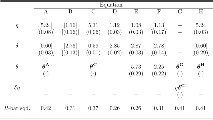
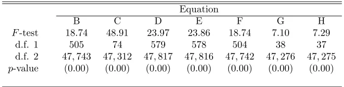
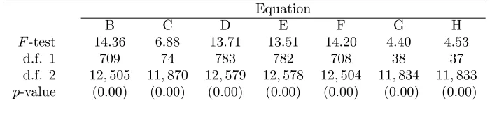
The disaggregate level trade estimation results for the benchmark case (i.e., the …rst approach in which zero trade observations are set equal to one U.S. dollar’s worth) are given in Table 2. Table 2 distinguishes between di¤erent versions of the estimated equation. As described above, versions B,C,D,E, F, and H are all restricted versions of version A, and version G is a special case of version A. Thus, these restrictions can be tested, and it can be decided whether or not they are valid. The test results for these restrictions are given in Table 3. As is evident, all the restrictions are rejected according to F-test results. This suggests that Version A, which is obtained through the model, is selected among all of versions. This implies that:
2 1Unfortunately, a tobit speci…cition cannot be employed to account for the zeros, because trade ratios rather than trade levels are
Source speci…c …xed e¤ects are found to be signi…cant in version B, which supports the assumption of source speci…c taste parameters in the utility function.
Trade costs are found to be good speci…c in version C, which supports the assumption of good speci…c trade costs.
Production technology for each good is found to be region speci…c in version G, which further supports the model.
Elasticity of substitution across varieties is found to be good speci…c in version H, which supports the disag-gregate level model.
As is evident by Version A in Table 2, the elasticity of substitution across regions is estimated as 5.24 on average.22 Since the intranational studies within the U.S. such as Wolf (2000), Hillberry and Hummels (2001), and
Millimet and Thomas (2007) use gravity equations, they cannot estimate for the elasticity of substitution and the elasticity of distance at the same time. So, the results in this paper are compared with the results in empirical international trade literature. It is found that the estimates of this paper for the elasticity of substitution are lower on average. In particular, Hummel’s (2001) estimates range between 4.79 and 8.26; the estimates of Head and Ries (2001) range between 7.9 and 11.4; the estimate of Baier and Bergstrand (2001) is about 6.4; Harrigan’s (1993) estimates range from 5 to 10; Feenstra’s (1994) estimates range from 3 to 8.4; the estimate by Eaton and Kortum (2002) is about 9.28; the estimates by Romalis (2007) range between 6.2 and 10.9; the (mean) estimates of Broda and Weinstein (2006) range between 4 and 17.3. This di¤erence may be due to the distinction between intranational and international data sets as well as the ignored factors in the literature such as local distribution costs, insurance costs, local taxes and intermediate input trade. Since the model of this paper controls for all of these factors, it can be claimed that we have more accurate results intranationally. Someone may claim that the di¤erence between the estimates of this paper and the estimates in the literature may also be due to the inclusion of zero trade observations; however, as it will be shown in the sensitivity analyses below, the di¤erence gets higher when zero trade observations are ignored, which is what the studies mentioned above actually do.
According to Version A in Table 2, the distance elasticity is estimated as 0.60 on average. This average value is higher than the distance elasticity estimates found by the literature, which are about 0.3 (see Hummels, 2001; Limao and Venables, 2001; Anderson and van Wincoop, 2004). This di¤erence is most probably again due to using di¤erent frameworks or data sets, as well as due to the inclusion of zero (trade) observations into the analysis. The latter possibility will be tested in the sensitivity analysis below. Another possible explanation for the di¤erence between the distance elasticity estimates of this paper and the ones in the literature may be the mode of transportation for interstate trade. In particular, it may well be the case that the interstate trade is done by air through couriers like UPS, FedEX, and so forth, while the international trade is done in transportation modes di¤erent from those. This possibility will also be considered by employing di¤erent distance measures in the sensitivity analysis below. Another reason may be the usual assumption of iceberg transport costs in the literature. As can be shown, if such an assumption is used instead of having a transportation sector, the distance elasticities would have had lower estimates.23 However, since the data set of CFS provides only the income received by the exporter …rms
(and excludes transportation income), it is distinguished between the exporter income and the transporter income, which is against the iceberg cost assumption.
Although version A (implied by the model) is selected among all estimated versions by the restriction tests, one can still have inference from other versions. Note that versions E and F represent the cases by which we can analyze whether or not there is a home-bias. Again according to Table 2, the values for H are positive and
signi…cant, which, according to the de…nitions of versions E and F, suggest that there is a home-bias across the states of the U.S. This bias is estimated as 5.73 by Equation E and 2.25 by Equation F. However, since Equation E is a restricted version of Equation F, one can further test this restriction. It is found that the restriction is rejected, which means that a home-bias of 2.25 is more plausible compared to 5.73. In particular, a typical state has a taste parameter for locally produced goods about 2.25 times more than imported goods. This number is very close to the intranational home-bias estimated by Hillberry and Hummels (2003) which isexp(0:99) = 2:69. Therefore, although the literature overestimates the elasticity of substitution measures and underestimates the elasticity of
2 2The individual estimated are available upon request. Also note that the estimates are highly signi…cant. Moulton (1986) suggests
that one should adjust the standard errors for OLS for the fact that the errors are correlated within the groups because of the common
group e¤ect. In this context, for robustness, we have also considered Moulton standard errors, and the (t-test) results are almost the
same. These results are also available upon request. See Moulton (1986) and Donald and Lang (2007) for the details of Moulton standard errors.
2 3It can be shown easily that the average (j)estimate given in Table 1 (i.e.,0.59) would be replaced by 0.43 under the iceberg cost
distance measures with respect to our results, the measures of home-bias seem to be similar. One explanation is due to the interaction between the two elasticity measures in Equation 4.3. In particular, if two elasticity measures operate in opposite signs (i.e., if one is overestimated and the other is underestimated), then the results for the …xed e¤ects captured by values are not a¤ected too much since two estimation errors cancel each other out to some degree.
Finally, the high adjustedR2value of 0.42 for Equation A also supports our model. Although version A (implied by the model) is selected among all estimated versions by our signi…cance tests, the contribution of each variable in Equation 4.3 can still be compared, in terms of explaining interstate trade patterns, by considering the adjustedR2
values of each version. In particular, the highest di¤erence of adjustedR2values takes place between versions A and D&E, which means that source speci…c …xed e¤ects and good speci…c trade costs together play an important role in the estimations. The second highest di¤erence of adjustedR2 values takes place between versions A and B&F, which means that source speci…c …xed e¤ects are signi…cant individually. The third highest di¤erence of adjusted
R2 values takes place between versions A and C, which means that good speci…c trade costs are also signi…cant
individually. Finally, the lowest di¤erence of adjustedR2 values takes place between versions A, G and H, which
means that good and region speci…c technology parameters and elasticities of substitution across goods, besides the source speci…c …xed e¤ects, play a lesser role compared to other parameters, which is reasonable since the empirical analysis is achieved within a highly integrated economy, the U.S.
5.1.1. Sensitivity Analyses
In order to support test the validity of the empirical results, four sensitivity analyses are employed in this section. The …rst two are related to zero (trade) observations, the third one is related to distance measures, and the last one is related to a possible biasedness of the OLS estimator in log-linearized models.
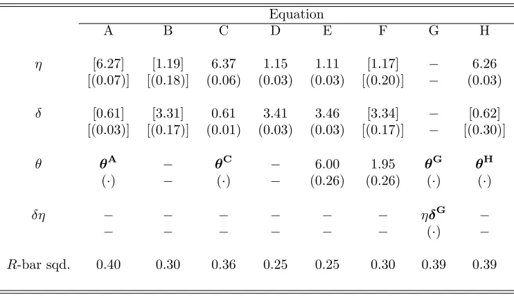
Sensitivity Analysis #1 We start the sensitivity analysis by setting zero (trade) observations equal to one U.S. cent’s worth. In such a case, the estimation results in Table 2 are replaced by the ones in Table 4. Note that the restrictions of versions B, C, D, E, F, G, and H can again be tested with respect to version A. The test results for these restrictions are given in Table 5. As is evident, all the restrictions are again rejected according to ourF-test results. This suggests that version A is again selected among all equations. The high adjustedR2value of 0.40 for Equation A again supports the model.
As is evident by Version A in Table 4, the elasticity of substitution is estimated as 6.27 on average. Although this average value is slightly higher than the ones in our benchmark case, they are still lower than the estimates in the literature on average.24
The distance elasticity is estimated as 0.61 on average, which is very close to the initial estimate in Table 2, yet higher than the ones in the literature.
Again according to Table 4, the values for H are positive and signi…cant, which according to the de…nitions
of versions E and F, suggest that there is a home-bias across the states of the U.S. After a restriction analysis between versions E and F, the restriction in E is rejected; thus, a typical state has a taste parameter for locally produced goods about 1.95 times more than imported goods. This number is close to the initial estimate of 2.25 in the benchmark case.
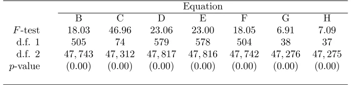
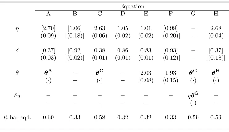
Sensitivity Analysis #2 For the second sensitivity analysis, the zero (trade) observations are ignored. In such a case, the estimation results in Table 2 are replaced by the ones in Table 6. The restrictions of versions B, C, D, E, F, G, and H are again tested with respect to version A. The test results for these restrictions are given in Table 7. As is evident, all the restrictions are again rejected according toF-test results. This suggests that version A is again selected among all equations. The high adjustedR2value of 0.60 for Equation A again supports the model.
This time, according to Version A in Table 6, the elasticity of substitution is estimated as 2.70 on average. This average value is very low compared to the studies mentioned above even though they also ignore zero trade observations (as in this subsection). We had given possible explanations for this di¤erence above, so we won’t repeat them here.
The distance elasticity is estimated as 0.37 on average. Although this average value is closer to the distance elasticity estimates in the literature (that we mentioned above, which are about 0.3), it is still relatively higher. Thus, the di¤erence between the …rst two estimates of distance elasticities (i.e., the estimates in the benchmark case and the …rst sensitivity analysis) and the estimates in the literature can, to some degree, be explained by the
inclusion of zero (trade) observations in the …rst two estimations. Nevertheless, the di¤erence doesn’t disappear completely.
According to Table 6, the values for H are again positive and signi…cant, which according to the de…nitions for
Equations E and F, suggest that there is a home-bias across the states of the U.S. In particular, a typical state has a taste parameter for locally produced goods about 1.93 times more than imported goods after testing for the restriction between Equations E and F and rejecting it. This number is lower compared to our initial estimates and the estimates of Hillberry and Hummels (2003).
Sensitivity Analysis #3 Until now, great circle distances have been used in the estimations, because average distance measures are not provided by CFS for zero (trade) observations. However, as is shown by Hillberry and Hummels (2001), using great circle distances, instead of actual distances provided by CFS, may overstate the distance measure as in Wolf (2000). In one of the remarks, we had claimed that we already control for this issue by taking the ratio of imports as the dependent variable. Moreover, the coe¢cient of correlation between the great circle distances and actual distances provided by CFS is calculated as0:98, after ignoring zero trade observations. Nevertheless, as the third sensitivity analysis, the sensitivity analysis #2 is repeated, this time using the average distance measure provided by CFS instead of the great circle distance measure that has been used until now. In this way, the e¤ects of great circle distances and the CFS distances can be compared.
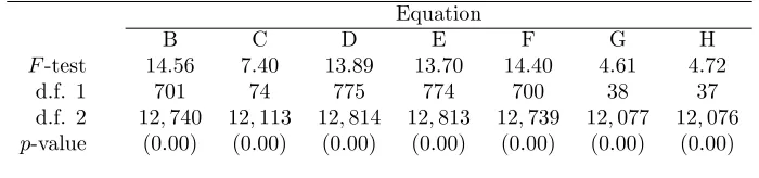
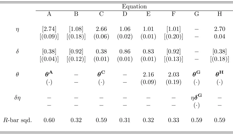
When CFS distances are used, the estimation results of sensitivity analysis #2 given in Table 6 are replaced by the ones in Table 8. The restrictions of versions B, C, D, E, F, G, and H are again tested with respect to version A. The test results for these restrictions are given in Table 9. As is evident, all the restrictions are again rejected according toF-test results. This suggests that version A is again selected among all equations. The high adjusted
R2value of 0.60 for Equation A again supports the model.
As is evident by Version A in Table 8, the elasticity of substitution is estimated as 2.74 on average. The distance elasticity is estimated as 0.38 on average. All of these estimates are very close to the ones presented for Sensitivity Analysis #2.
According to Table 8, the values for H are again positive and signi…cant, which, according to the de…nitions of
Equations E and F, suggest that there is a home-bias across the states of the U.S. In particular, a typical state has a taste parameter for locally produced goods about 2.03 times more than imported goods after testing for the restriction between Equations E and F, and rejecting it. Although this number is close to our initial estimates, it is slightly higher compared to Table 6.
Overall, the numbers in Table 6 and Table 8 are not signi…cantly di¤erent from each other. This result supports the claim that overstating distances mentioned by Hillberry and Hummels (2001) is already controlled for in this paper.
Sensitivity Analysis #4 For the last sensitivity analysis, the benchmark case and the …rst three sensitivity analyses are repeated by using Poisson Pseudo-Maximum Likelihood (PPML) estimator. As Santos Silva and Tenreyro (2006), and Henderson and Millimet (2008) suggest, under heteroskedasticity, the parameters of log-linearized models estimated by OLS may lead to biased estimates; thus, PPML should be used. To show this, Equation 4.3 can be written as follows:
Xr;a(j)
Xr;b(j)
= exp log a
b
+ ( (j) 1) log Aa(j)
Ab(j)
+ (j) (j) log Dr;b
Dr;a
r;a;b;j (5.1)
AssumingE[ r;a;b;jj ab;AAab((jj));DDr;ar;b] = 1, then Equation 5.1 may be estimated consistently using the Poisson
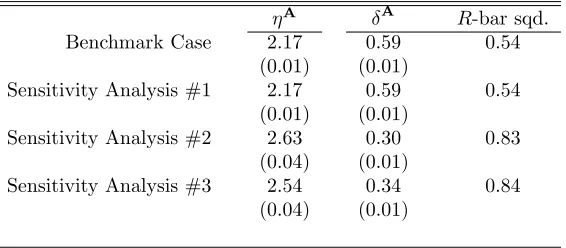
Pseudo-Maximum Likelihood (PPML) estimator (see Santos Silva and Tenreyro, 2006). Since Version A has been chosen among all versions earlier, we repeat our analysis only for Version A here. The results are given in Table 10.
As is evident, the (average) elasticity of substitution across varieties ranges between 2:17and 2:63, and the (average) elasticity of distance ranges between0:30and0:59, which are both consistent with our earlier claim that our estimates are lower than and our estimates are higher than the ones in the international trade literature.
5.2. Aggregate Level Trade Estimation Results
2:19by PPML). When zero trade observations are ignored, it is estimated as 1:95 by OLS (respectively, 2:44 by PPML). Finally, when CFS distance measures are used instead of great circle distances, it is estimated as1:92by OLS (respectively,2:97by PPML).
Although the estimates of"are lower than the elasticity of substitution across varieties estimates (i.e., (j)’s), as expected, according to OLS estimator, they are very close to each other according to PPML estimator. This result is consistent with the view that when goods are aggregated, the elasticity of substitution across them decreases. Nevertheless, these numbers are signi…cantly lower than the estimates in the literature that were discussed above. As in the disaggregate level analysis, we claim that this di¤erence may be due to distinction between intranational and international data sets as well as the ignored factors in the literature such as local distribution costs, insurance costs, local taxes and intermediate input trade. Since the model of this paper controls for all of these factors, we claim that we have more accurate results intranationally. The results are further supported by several sensitivity analyses with high explanatory powers.25
6. Conclusions
This paper has introduced a partial equilibrium model to …nd motivations for bilateral trade ratios across regions. It is shown that a region imports more goods from the higher technology regions and fewer goods from the more distant regions, subject to an elasticity of substitution across varieties. Moreover, a region imports more of a good, of which price is lower, subject to an elasticity of substitution across goods. When bilateral trade is estimated in ratio form (rather than in levels), the model of this paper has several empirical and analytical bene…ts compared to the gravity models, which are explained in details in the text. Thanks to the disaggregate (state) level data set combined from the Commodity Flow Survey and the U.S. Census Bureau, it is found that the simple model of this paper is capable of explaining the interstate trade patterns within the U.S. It is also shown that the elasticity of substitution measures are overestimated in the literature, while the elasticity of distance measures (thus, trade costs) are underestimated in the literature relative to the estimates of this paper.
It has been also shown that source speci…c …xed e¤ects and good speci…c taste parameters are important for bilateral trade patterns, which are usually ignored in the literature. Moreover, elasticities of substitution across varieties and trade costs are good speci…c, which is not a considered fact in most of the aggregate level gravity type studies. Besides, production technology for each good is found to be region speci…c rather than country speci…c. Several sensitivity analyses support these results.
The best strategy for possible future research would be to extend the model of this paper toward explaining international trade patterns. Such an analysis would be more convenient with a general equilibrium framework, although a partial equilibrium framework was su¢cient for this paper.
2 5We have also tested di¤erent restricted versions of Equation 4.6, such as common ’s or common P
i(j)’s, in our aggregate level