Enhancing Retrieval of Geological Text using Named Entity Disambiguation

(1)

International Journal of Emerging Technology and Advanced Engineering

Website: www.ijetae.com (ISSN 2250-2459, Volume 2, Issue 1, January 2012)

269

Enhancing Retrieval of Geological Text using Named

Entity Disambiguation

Sobhana N.V

1

Associate Professor, Dept of Computer Science and Engg, Rajiv Gandhi Institute of Technology, INDIA.

[email protected]

Abstract— The paper presents a comparative study of performance of different information retrieval models and co-occurrence based place name disambiguation and query expansion on a geological text corpus. As an initial step, we have created a moderate sized corpus containing documents pertaining to geology of the Indian subcontinent and performed indexing and retrieval on the collection. The different retrieval models considered are TF-IDF, BM25, InL2, PL2, IFB2, BB2, InexpB2 and InexpC2. After this a co-occurrence graph based disambiguation algorithm to resolve ambiguities in place names in the corpus is introduced. After disambiguation, using neighborhoods in the co-occurrence graph, the query can be expanded with related place names. Our experiments on a Geological corpus (IITKGP-GEOCORP) show that query expansion with place disambiguation performs significantly better than baseline method.

Keywords—

Geological corpus; precision; recall; Co-occurrence matrix; Co-Co-occurrence graph (key words)

I.INTRODUCTION

Geological documents pertain to data concerning geological objects distributed over a large span of space and time. Geological data utililizes spatial references as well as georeferences in text. The presence of additional time dimension in the geological documents leads to additional complexities like evolution of location names over the temporal co-ordinates and change in geo references over time. Geological documents contain geospatial and temporal information i.e., it represents geological data spread over space and time. The documents also contain information pertaining to various places ranging from oceans to the various continents thus spanning a large space. Time and locational references are often interdependent and form a complex referencing scheme. E.g. Gondwana land is a Precambrian name of the present Deccan Region of South Asia.

It is important to mine geological data for the information that they both represent the same region. Otherwise information about Gondwana land that is available is not being used for the study of Deccan Region.

One of the main challenges in processing of natural language text is ambiguity. Information retrieval systems which lack of disambiguation capability often suffer in performance. The expanding of query with intended synonyms and toponyms after disambiguation, can improve retrieval performance.

Term co-occurrence model is based on the hypothesis that, in a sufficiently large corpus if some terms appear frequently in the same co-occurrence window, then there exists semantic relations between them. For higher co-occurrence frequency, semantic relations becomes stronger. Term co-occurrence has been used in many language processing tasks such as information retrieval, natural language processing and computational linguistics etc [1].

Co-occurrence models have been used by Overell and Ruger for place name disambiguation. They showed that the disambiguation of polynyms and synonyms, leads to improve results in geographical information retrieval [2][3][4]. Andogah and Bouma implemented a complete place name ambiguity resolution system consisting of three components: geographical tagger, geographical scope resolver (GeoSR) and place name referent resolver (PRR) [5]. Smith and Crane implemented the toponym disambiguation system in the Perseus digital library and evaluated its performance [6].

(2)

International Journal of Emerging Technology and Advanced Engineering

270

Voorhees has used Wordnet in determining expansion terms [8]. She performed experiments on TREC collection and expanded query using a combination of synonyms and hyponyms from Wordnet. The important factor that determines the effect of query expansion is the selection of appropriate expansion terms [9]. Bai, Nie and Cao used context dependent term relations for better expansion terms. They showed that Context dependent relations obtained by adding context word to the relation, performs much better than the co-occurrence relations [7].

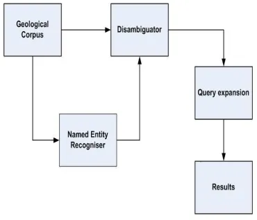
[image:2.612.82.267.374.533.2]

Word co-occurrence matrix and graph are introduced in this work to represent strong mutual relationships between place names. We introduce a graph based disambiguation algorithm to resolve ambiguities such as reference ambiguity and referent ambiguity in place names. After disambiguation, using neighborhoods in the co-occurrence graph, the query can be expanded with related place names. The overall schema of the system is shown in figure I.

Figure I:The Schema of the Retrieval System

II.CO-OCCURRENCE BASED NAME DISAMBIGUATION

Co-occurrence based disambiguation system builds up a term co-occurrence model that captures co-occurrence information of places from a corpus. It includes occurrence matrix and occurrence graph. The co-occurrence matrix and graph represent the places and order in which they occur. They also reveal the relationship between different places. The number of times, the place names co-occur together is represented by co-occurrence matrix. Each node in the co-occurrence graph corresponds to place names and edge represents how they co-occur.

Co-occurrence is computed for words appearing together in a sentence, within a window of n words or in a document. We exploit term co-occurrences in our problem. Terms do not necessarily co-occur side by side. They often appear at some distance of each other. The following formula is used to determine the probability of term co-occurrences in a biterm model.



i j i j

i j wi

c

(

w

,w

)

P

(

w

|w

)

=

c

(

w

,w

)

(1)

where c(wi,wj)is the frequency of co-occurrence of the

biterm (wi,wj), i.e, two terms in the same window of fixed

size across the collection.[ 10].

The degree of biases of co-occurrence can be

computed using



2 test. If term frequency is small, the degree of biases are not reliable. As an example let term t1

appear lesser number of times and co-occur with term r. Let term t2 appear more number of times and co-occur with

term r. Then term t2 is more reliably biased to r. For

evaluating statistical significance of biases



2 test is used. It is used for evaluating biases between expected frequencies and observed frequencies. The unconditional probability of a frequent term s



S is the expected probability ps and the total number of co-occurrence of

term v and frequent terms S as nv. The frequency of

co-occurrence of term v and term s is freq(v,s). The statistical value of



2 isdefined as



vs2

2

vs sεS

(

f

r

e

q

(

v

,

s

)

-

n

p

)

ψ

(

v

)

=

n

p

(2)

nvps represents the expected frequency of

co-occurrence. (freq(v,s)-nvps ) represents the difference

(3)

International Journal of Emerging Technology and Advanced Engineering

271

India Delhi West Bengal

Maharas tra

Karn ataka

Tamil nadu

India ₀ ₄₈ ₂₄ ₂₀ ₂₈ ₂₆

Delhi ₄₈ ₀ ₅ ₃ ₂ ₂

West Bengal

24 5 0 3 2 2

Mahara shtra

20 3 3 0 2 3

Karnat aka

28 2 2 2 0 4

Tamil nadu

26 2 2 3 4 6

We define a co-occurrence graph, G(V,E) (V is the set of nodes and E is the set of edges) as a directed graph from the co-occurrence matrix. Each node p represents place names. An edge eij є E is created between two nodes pi,pj if

[image:3.612.58.276.484.625.2]

they co-occur. ie an edge is formed between two nodes if place names represented by those nodes co-occur. The graph represent the direct and indirect relationship between place names. A node which lies n hops away from node p has n order co-occurrence with the node p.

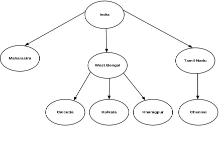
Figure II. Typical Co-occurrence graph

Using Breadth First Search on the co-occurrence graph we can search each node and the query can be expanded using neigbouring nodes. For example, the West Bengal node explores as Kharagpur, Calcutta, Kolkata etc. Thus using the co-occurrence graph the query can be expanded using synonyms of place names.

Place name ambiguities are either referent ambiguity or reference ambiguity. Referent ambiguity occurs when the same place name is used for several locations. Reference ambiguity occurs when the same location has multiple names. The

sense

of a place name (i.e.

meaning

) is used when the place name has a number of distinct meanings.

Methodology for handling referent ambiguity for a given context

Step 1: Select next ambiguous toponym tp having

sn senses;

Step 2: Find subhierarchies one for each sense of

sn;

Step 3: Select the ambiguous node in each subhierarchy of each sense; let it be node_a and

node_b;

Step 4: Find the co-occurrence count of node_a

and node_b; let it be count_a and count_b;

Step 5: if count_a ≠ count_b, select sense having context and higher co-occurrence count.

Step 6: if count_a = count_b, compare ancestor of

(node_a) and ancestor of (node_b) with context

for finding the correct sense.

For example consider Kharagpur in Bengal and Kharagpur in Bihar. From such ambiguous place names different sub hierarchies are formed in the graph. This is shown in figure II. Let the co-occurrence count of Kharagpur in West Bengal be higher compared to the co-occurrence count of Kharagpur in Bihar. Then Kharagpur in West Bengal is selected. If the co-occurrence count of Kharagpur in Bihar is low ie, below a threshold value, it is not considered for disambiguation.

Methodology for handling reference ambiguity for a given context

Step 1 : select next ambiguous synonym sm having sn

senses;

Step 2 : find subhierarchies one for each sense of sn;

India

West Bengal

Kolkata Calcutta

Maharastra _{Tamil Nadu}

(4)

International Journal of Emerging Technology and Advanced Engineering

272

Step 3 : select node in each subhierarchy of each sense; let it be node_a and node_b;

Step 4 : Find the subtree in the next level of node_a and

node_b; let it be subtree_a and subtree_b;

Step 5 : if subtree_a = subtree_b and ancestor of

(node_a) = ancestor of (node_b), sense

related to node_a and sense related to

node_b are synonyms.

For example, when Calcutta and Kolkata appear in the graph, compare the nodes in the next level of Calcutta with the nodes in the next level of Kolkata. If the number of node matches is above the threshold value then Calcutta is a synonym of Kolkata. Thus the query can be expanded with Calcutta, Kolkata etc. Another method to deal with referent ambiguity is, consider Calcutta and Kolkata in the context in which they appear. In the corpus there exist statements such as Calcutta or Kolkata, Calcutta (Kolkata), Calcutta is known as Kolkata etc . Each of these statements implies that Calcutta is a synonym of Kolkata.

III. QUERY EXPANSION USING CO-OCCURRENCE GRAPH

Query expansion is the process of expanding user’s query with additional or new terms in order to improve results. The new terms can either be statistically related to the original query words (ie, terms tend to co-occur with one another in documents) or chosen from lexical aids such as thesauri. In this work, query expansion utilizes word co-occurrence. Words co-occuring in a document or paragraph are likely to be in some sense similar or related in meaning. The advantage of co-occurrence analysis lies in the fact that information is easily generated from the documents and requires no human intervention. The selection of expansion terms is done by exploiting hierarchical relationships in co-occurrence graph and also by making use of synonyms. For example, Maharashtra is expanded with Mumbai, Bombay, Nagpur, Pune etc. The query expansion is described below.

Input: Firstnode, N, GEOQUERY //Firstnode is the starting vertex of co-occurrence graph. Let N be the number of vertices in the co-occurrence graph. GEOQUERY is a pointer to a list.

Output: VISIT //An array to store the order of visit of vertices during traversal.

Data structure: GEOQUEUE, Adjacency Matrix, Geographptr //The queue GEOQUEUE holds the vertices which is initially empty. Adjacency Matrix representation of graph. Geographptr is the pointer to graph.

If (Geographptr = NULL) then

Print “Graph is empty”

Exit

EndIf

Currentnode = Firstnode

QUEUE.INSERT_QUEUE(Currentnode) // Enter the starting vertex into the QUEUE

While(GEOQUEUE.STATUS() ≠ EMPTY) do // //Till the GEOQUEUE is not empty

Currentnode= GEOQUEUE.DELETE_QUEUE()

// Delete an item from QUEUE

If (SearchArray(GEOVISIT, Currentnode) =

FALSE) then

// If Currentnode is not in the array

//GEOVISIT

InsertArray(GEOVISIT, Currentnode )

//Store visited node Snode in VISIT

If Currentnode = “geolocation”

// If Currentnode is a particular place, say

// West Bengal

For i = 1 to N do

(5)

International Journal of Emerging Technology and Advanced Engineering

273

GEOQUERY = GEOQUERY U i

// Original query is expanded

// with children of Currentnode

Endif

EndFor

else

For i = 1 to N do // To enter all adjacency

//vertices of Snode into QUEUE

If (Geographptr[Node][i] = 1) then

QUEUE.INSERT_QUEUE(i)

EndIf

EndFor

EndIf

EndWhile

Return

Stop

This algorithm begins at the root node of co-occurrence graph, explores the neighbouring nodes and expands the query using them. For example. if the Currentnode is West Bengal, the GEOQUERY is expanded with Calcutta, Kolkata and Kharagpur. It make use of queue data structure GEOQUEUE and adjacency matrix. GEOVISIT stores the traversal order of visited vertices. We have used a few operations on the queue such as INSERT_QUEUE and DELETE_QUEUE.

In this work, Named Entity Recogniser recognizes georeferences ie, location names. The machine learning technique (conditional random fields) is used to prepare baseline classifier using the annotated data and features. We have used the C++ based OpenNLP CRF++ package for named entity recognition [13]. For evaluation of retrieval performance we have used the open source Terrier

(TERabyte RetRIEveR) IR platform,

(

http://ir.dcs.gla.ac.uk/terrier

) as implementations of the

retrieval models [14].

IV. EVALUATION METHODOLOGY

We use the classic Precision and Recall as the measures used in evaluating information retrieval strategies. Let number of relevant documents in the collection be Nrc. Let

the number of documents retrieved be Nrd and the number

of documents retrieved which are relevant be Nr. Then

precision and recall may be defined as:

r

rd

N

P

re

c

isio

n

N



(3)

r

rc

N

Recall

N



(4)

A combined measure called F-measure which is dependent on both Precision and Recall is also commonly used. It reflects importance of Recall versus Precision.

1

1 F

P

r

e

c

i

s

i

o

n R

e

c

a

l





(5)

We calculate the precision and recall at different values of Nrt e.g.,1, 5, 10, 20, 30 etc We also calculate the Mean

(6)

International Journal of Emerging Technology and Advanced Engineering

274

V. GEOLOGICAL CORPUS

The Geological corpus (IITKGP-GEOCORP) was created out of a collection of scientific reports and articles on the geology of the Indian subcontinent. Many of these constituted reports submitted to the Earth Sciences Division of Department of Science and Technology, Government of India. The corpus consists of about 500 documents with each document about 10,000 words long, representing various aspects of geology. The lexicon consisted of several well known as well as rare geological terms. The titles of some of these documents are listed below.

TABLE II:TYPICAL DOCUMENT TITLES IN THE IITKGP-GEOCORP

Coastal Forms and Processes of the Godavari Delta Retreat of Himalayan Glaciers: Indicator of Climate Change

Metamorphism of the Oddanchatram Anorthosite, Tamil Nadu, South India

K-T magmatism and basin tectonism in western Rajasthan, India, results from extensional tectonics and not from Reunion plume activity

Crustal geotherm in southern Deccan Basalt Province, India: The Moho is as cold as adjoining cratons

Erosion and sedimentation in Kalpakkam (N Tamil Nadu, India) from the 26th December 2004 tsunami

Grain-size distribution, morphoscopy and elemental chemistry of suspended sediments of Pindari Glacier, Kumaon Himalaya, India

We also considered over 100 queries based on the feedback of a pool of the geological researchers. We have manually constructed a set of relevance judgments for all these documents in the corpus with help of the experts in Indian Subcontinent Geology. Some of the queries are listed below.

TABLE III:SAMPLE QUERIES

narmada

gondwana

karakoram

western ghats

damodar valley

thar desert

VI. INFORMATION RETRIEVAL MODELS

In this section we briefly mention some of the information retrieval models. Each model is associated with a scoring function which is used for relevance ranking. All these functions represent some kind of inner product for vector space representation of the documents using term frequencies (TF) and inverse document frequencies (IDF). Appropriate normalizations and randomness are introduced in the weights by different models.

TF-IDF(Term Frequency Inverse Document Frequency)

model works by determining the relative frequency of words in a specific document compared to the inverse proportion of that word over the entire document corpus.

Okapi BM25: is a ranking function used by search

engines to rank matching documents according to their relevance to a given query. It is a probabilistic model.

InL2: Inverse document frequency model for

randomness, Laplace succession for first normalisation, and Normalisation 2 for term frequency normalisation.

PL2: Poisson estimation for randomness, Laplace succession for first normalisation, and Normalisation 2 for term frequency normalisation.

In_expB2: Inverse expected document frequency model

for randomness, the ratio of two Bernoulli's processes for first normalisation, and Normalisation 2 for term frequency normalisation.

DFR_BM25: The divergence from random DFR version

(7)

International Journal of Emerging Technology and Advanced Engineering

275

IFB2: Inverse Term Frequency model for randomness,

the ratio of two Bernoulli's processes for first normalisation, and Normalisation 2 for term frequency normalisation.

BB2: Bose-Einstein model for randomness, the ratio of two Bernoulli's processes for first normalisation, and Normalisation 2 for term frequency normalisation.

In_expC2: Inverse expected document frequency model

for randomness, the ratio of two Bernoulli's processes for first normalisation, and Normalisation 2 for term frequency normalisation with natural logarithm.

VII. EXPERIMENTAL RESULTS

A. Comparative Study of Different Retrieval Models

In Table IV we present the precision obtained by different models on the corpus. Gold standard was provided by human relevance judgment. The average value over 100 queries are reported. Note that precision values are presented for different numbers of retrieved documents (Nrt

= 1, 5, 30 etc).

It has been observed that BB2 model has higher precision as compared to other models and PL2 model has lower precision than other models.It is also been observed that precision values of TF-IDF is better than IFB2, In-expB2, InL2, PL2 and comparatively it is higher for DFR-BM25, BB2, In-expC2.

The mean average precision (MAP) is also presented in Table VI. We observe that TF-IDF and BM25 models have higher average mean precision than other models. This agrees with the theoretical expectations. It is also been observed that mean average precision values of TF-IDF are better than IFB2, In-expB2, InL2, PL2, DFR-BM25, BB2 and In-expC2.

B. Comparative Study of Different Retrieval Models with Query Expansion

In Table VII we present the precision values obtained by different models on the corpus. Gold standard was provided by human relevance judgment. The average value over 100 queries are reported. Similarly Table VIII shows the recall scores.

Note that precision is presented for different numbers of retrieved documents (Nrt = 1, 10, 30 etc). It is observed that

PL2 model has higher precision values than other models and BB2 model has lower precision values than other models. It is also been observed that precision values of TF-IDF are better than BB2, In-expB2, In-expC2 and comparatively it is higher for DFR-BM25, IFB2, InL2,PL2.

The mean average precision (MAP) is also presented in Table IX. The Mean Average Precision (MAP) is also presented in Table VI. We observed that BM25 model has higher Mean Average Precision than other models. InL2 model has lower Mean Average Precision than other models. It is observed that BM25 model has highest mean average precision than other models and InL2 model has the lowest mean average precision than other models. This agrees with the studies found in the literature for geographical text. It is also been observed that mean average precision values of TF-IDF are better than BB2, IFB2, In-expB2, In-expC2, InL2 and comparatively it is higher for BM25, DFR-BM25, PL2.

TABLE VI:MEAN AVERAGE PRECISION

Retrieval models

MAP

BM25 0.8610

DFR_BM25 0.8560

TF_IDF 0.8610

InL2 0.8540

PL2 0.8547

InexpB2 0.8540

BB2 0.8456

IFB2 0.8555

InexpC2 0.8560

(8)

International Journal of Emerging Technology and Advanced Engineering

276

TABLE IV : PRECISION VALUES

InL2 PL2 In_expB2 DFR_BM25 BB2 BM25 TF-IDF IFB2 In_expC2

1 0.6167 0.5633 0.6167 0.5833 0.5976 0.5833 0.5833 0.5722 0.5833

5 0.7925 0.8131 0.7925 0.8183 0.8167 0.8173 0.8173 0.8183 0.8183

30 0.8965 0.8852 0.8965 0.8855 0.8831 0.8724 0.8776 0.8517 0.8841

75 0.3125 0.3125 0.3125 0.3125 0.3125 0.3168 0.3168 0.3125 0.3125

110 0.8056 0.8056 0.8056 0.9167 0.9167 0.9167 0.9167 0.9167 0.9167

TABLE VII: PRECISION VALUES

Nrt BM25

DFR-BM25

TF-IDF BB2 IFB2 InexpB2 InexpC2 InL2 PL2

1 0.8439 0.8468 0.8811 0.7512 0.8043 0.7775 0.7751 0.8658 0.9144

10 0.8060 0.8120 0.8060 0.7794 0.8976 0.7950 0.7947 0.8236 0.9448

30 0.5992 0.6025 0.6131 0.5523 0.6229 0.5873 0.5908 0.6075 0.7708

50 0.8831 0.9043 0.9043 0.7839 0.7151 0.6954 0.6927 0.9096 0.9683

80 0.7212 0.7212 0.7212 0.7731 0.7731 0.7731 0.7212 0.7212 0.6879

100 0.7889 0.7889 0.7889 0.6227 0.8702 0.7460 0.7460 0.7889 0.7889

TABLE IX :MEAN AVERAGE PRECISION

Retrieval models MAP

BM25 0.9790

DFR_BM25 0.9560

TFIDF 0.9550

BB2 0.9110

IFB2 0.9520

InexpB2 0.9440

InexpC2 0.9460

InL2 0.9010

PL2 0.9560

(9)

International Journal of Emerging Technology and Advanced Engineering

277

The Co-occurrence based query expansion significantly improved the retrieval performance. It has been found that the Mean Average Precision of a system with query expansion is higher compared to a baseline system with no query expansion. Experimental results of the system with query expansion show 8.9% improvement when compared to the baseline system.

Comparison of Baseline and co-occurrence methods

0.75 0.8 0.85 0.9 0.95 1

BM 25

DFR -BM

25 TF

-ID F

BB 2

IFB 2

Inex pB2

Inex

pC2 InL2 PL2

Retrieval Models

M

e

an

A

ve

r

age

P

r

e

c

is

ion

Baseline Co-occurrence

VIIICONCLUSIONS

We have presented a study on evaluation and comparison of different retrieval algorithms on a Geological corpus. We proposed a Co-occurrence graph based method of query expansion with place disambiguation. We created a co-occurrence graph to represent place names, relationships and resolved the problem of place name ambiguity. The results showed that co-occurrence based query expansion with resolving place name ambiguity has improved the retrieval performance. Query expansion with relevance feedback mechanisms can be explored as extension of this work. Earlier version of this paper is available in [12]

References

[1] Nan Q. Y., Yong Q. and Di H. 2009 A Study on unified Term

Co-occurrence Model, Information Technology Journal, pp. 1033-1038.

[2] Overell S. E. and Ruger S. M, 2008 Using co-occurrence models

for place name disambiguation, International Journal of Geographical Information Science, 22 (3), pp. 265-287.

[3] Overell S. E., Ruger S. M, 2007 Forostar: A system for GIR,

Springer Verlag Berlin Heidelberg LNCS 4730, pp. 930-937.

[4] Overell S. E., Ruger S. M, 2006 Identifying and grounding

descriptions of places, In:SIGIR Workshop on Geographic Information Retrieval.

[5] Andogah G., Bouma G., Nerbonne J., Koster E., 2008

Geographical Scope Resolution, Workshop at the 6th Conference on Language Resources and Evaluation (LREC), Paris, pp. 4-10.

[6] Smith D. A., Crane G., 2001 Disambiguating Geographic Names

in a Historical Digital Library, Springer-Verlag Berlin Heidelberg,

LNCS 2163, pp.127–136.

[7] Bai J., Nie J. Y., Cao G., 2006 Context Dependent Term Relations

for Information Retrieval, Information Retrieval Proceedings of the 2006 Conference on Empirical Methods in Natural Language Processing (EMNLP 2006), Sydney, pp. 551–559.

[8] Voorchees E. M. 1994 Query Expansion using Lexical-semantic

Relations, In SIGIR '94: Proceedings of the 17th annual international ACM SIGIR conference on Research and development in information retrieval, pp. 61-69.

[9] Peat H. J., Willett P. 1991 The limitations of term co-occurrence

data for query expansion in document retrieval systems, JASIS, 42(5), pp. 378-383.

[10] Bai J., Nie J. Y, Cao G. 2006 Context Dependent Term Relations for Information Retrieval, Information Retrieval

Proceedings of the 2006 Conference on Empirical Methods in Natural Language Processing (EMNLP 2006), Sydney, pp. 551– 559.

[11] Matsuo Y., Ishizuka M 2004 Keyword extraction from a single

(10)

International Journal of Emerging Technology and Advanced Engineering

278

[12] Sobhana N. V, Alimpan Barua, Monotosh Das, Pabitra Mitra, Ghosh S. K, 2010, Co-occurrence based place name disambiguation and its application to retrieval of geological text, In Recent Trends in networks and communications, volume 90 of communications in computer and Information Science, 2010, 543-552, Springer Berlin Heidelberg.

[13] Taku Kudo. CRF++ 2005 an open source toolkit for CRF, http://crfp.sourceforge.net.