BIROn - Birkbeck Institutional Research Online
Chun, C. and Moffatt, I. and Noble, Steven and Rueckriemen, R. (2018) On
the interplay between embedded graphs and delta-matroids. Proceedings of
the London Mathematical Society , ISSN 0024-6115. (In Press)
Downloaded from:
Usage Guidelines:
On the interplay between embedded graphs and delta-matroids
∗
C. Chun
†, I. Moffatt
‡, S. D. Noble
§, R. Rueckriemen
¶August 31, 2018
Abstract
The mutually enriching relationship between graphs and matroids has motivated discoveries in both fields. In this paper, we exploit the similar relationship between embedded graphs and delta-matroids. There are well-known connections between geometric duals of plane graphs and duals of matroids. We obtain analogous connections for various types of duality in the literature for graphs in surfaces of higher genus and delta-matroids. Using this interplay, we establish a rough structure theorem for delta-matroids that are twists of matroids, we translate Petrie duality on ribbon graphs to loop complementation on delta-matroids, and we prove that ribbon graph polynomials, such as the Penrose polynomial, the characteristic polynomial, and the transition polynomial, are in fact delta-matroidal. We also express the Penrose polynomial as a sum of characteristic polynomials.
MSC Classification 05B35 (primary), 05C10, 05C31, 05C83(secondary).
1
Overview
Graph theory and matroid theory are mutually enriching. As reported in [29], Tutte famously ob-served that, “If a theorem about graphs can be expressed in terms of edges and circuits alone it probably exemplifies a more general theorem about matroids”. In [14] we proposed that a similar claim holds true for topological graph theory and delta-matroid theory, namely that, “If a theorem about embedded graphs can be expressed in terms of its spanning quasi-trees then it probably exem-plifies a more general theorem about delta-matroids”. In that paper we provided evidence for this claim by showing that, just as with graph and matroid theory, many fundamental definitions and results in topological graph theory and delta-matroid theory are compatible with each other (in the sense that they canonically translate from one setting to the other). A significant consequence of this connection is that the geometric ideas of topological graph theory provide insight and intuition into the structure of delta-matroids, thus pushing forward the development of both areas. Here we provide further support for our claim above by presenting results for delta-matroids that are inspired by recent research on ribbon graphs.
We are principally concerned with duality, which for delta-matroids is a much richer and more varied notion than for matroids. The concepts of duality for plane and planar graphs, and for graphic matroids are intimately connected: the dual of the cycle matroid of an embedded graph corresponds to the matroid of the dual graph (i.e.,M(G)∗=M(G∗)) if and only if the graph is plane. Moreover, the dual of the cycle matroid of a graph is graphic if and only if the graph is planar. The purpose of
∗Accepted for publication in the Proceedings of the London Mathematical Society.
†Mathematics Department, United States Naval Academy, Annapolis, Maryland, 21402-5002, United States of America,[email protected].
‡Department of Mathematics, Royal Holloway, University of London, Egham, Surrey, TW20 0EX, United Kingdom,
§Department of Economics, Mathematics and Statistics, Birkbeck, University of London, London, WC1E 7HX, United Kingdom,[email protected].
¶Aschaffenburger Strasse 23, 10779 Berlin,
this paper is to extend these fundamental graph duality–matroid duality relationships from graphs in the plane to graphs embedded on higher genus surfaces. To achieve this requires us to move from matroids to the more general setting of delta-matroids.
Moving beyond plane and planar graphs opens the door to the various notions of the “dual” of an embedded graph that appear in the topological graph theory literature. Here we consider the examples of Petrie duals and direct derivatives [35], partial duals [13] and twisted duals [16]. We will see that these duals are compatible with existing constructions in delta-matroid theory, including twists [5] and loop complementation [9]. We take advantage of the geometrical insights provided by topological graph theory to deduce and prove new structural results for delta-matroids and for their polynomial invariants.
Much of the very recent work on delta-matroids appears in a series of papers by Brijder and Hoogeboom [9, 10, 11, 12], who were originally motivated by an application to gene assembly in one-cell organisms known as cilliates. Their study of the effect of the principal pivot transform on symmetric binary matrices led them to the study of binary delta-matroids. As we will see, the fundamental connections made possible by the abstraction to delta-matroids allows us to view notions of duality in the setting of symmetric binary matrices and the apparently unconnected setting of ribbon graphs as exactly the same thing.
The structure of this paper is as follows. We begin by reviewing delta-matroids, embedded graphs and their various types of duality, and the connection between delta-matroids and embedded graphs. Here we shall describe embedded graphs as ribbon graphs (ribbon graphs are equivalent to graphs cellularly embedded in surfaces). In Section 3 we use the geometric perspectives offered by topological graph theory to present a rough structure theorem for the class of delta-matroids that are twists of matroids. We give some applications to Eulerian matroids, extending a result of Welsh [33]. In Section 4, we show that Petrie duality can be seen as the analogue of a more general delta-matroid operation, namely loop complementation. We show that a group action on delta-matroids due to Brijder and Hoogeboom [9] is the analogue of twisted duality from Ellis-Monaghan and Moffatt [16]. We apply the insights provided by this connection to give a number of structural results about delta-matroids. In Section 5 we apply our results to graph and matroid polynomials. We show that the Penrose polynomial and transition polynomial [1, 17, 24, 31] are delta-matroidal, in the sense that they are determined (up to a simple pre-factor) by the delta-matroid of the underlying ribbon graph, and are compatible with Brijder and Hoogeboom’s Penrose and transition polynomials of [10]. We relate the Bollob´as–Riordan and Penrose polynomials to the transition polynomial and find recursive definitions of these polynomials. Finally, we give a surprising expression for the Penrose polynomial of a vf-safe delta-matroid in terms of the characteristic polynomial.
Throughout the paper we emphasise the interaction and compatibility between delta-matroids and ribbon graphs. We provide evidence that this new perspective offered by topological graph theory enables significant advances to be made in the theory of delta-matroids.
2
Background on delta-matroids
2.1
Delta-matroids
A set system is a pair D = (E,F) where E is a non-empty finite set, which we call the ground set, andF is a collection of subsets ofE, calledfeasible sets. We defineE(D) to beE and F(D) to be
F. A set system (E,F) isproper if F is not empty; it istrivial if E is empty. For sets X and Y, theirsymmetric difference is denoted byX4Y and is defined to be (X∪Y)−(X∩Y). Throughout this paper, we will often omit the set brackets in the case of a single element set. For example, we writeE−einstead ofE− {e}, orF∪einstead ofF∪ {e}.
Adelta-matroidis a proper set systemD= (E,F) that satisfies the Symmetric Exchange Axiom:
Note that we allowv=uin the Symmetric Exchange Axiom. These structures were first studied by Bouchet in [5]. If all of the feasible sets of a delta-matroid are equicardinal, then the delta-matroid is amatroid and we refer to its feasible sets as itsbases. If a set system forms a matroidM, then we usually denoteM by (E,B), and defineE(M) to beE andB(M) to beB, the collection of bases of
M. Every subset of every basis is anindependent set. For a setA⊆E(M), therank of A, written
rM(A), or simply r(A) when the matroid is clear, is the size of the largest intersection of A with a
basis ofM.
For a delta-matroid D = (E,F), let Fmax(D) and Fmin(D) be the set of feasible sets with
maximum and minimum cardinality, respectively. We will usually omitD when the context is clear. Let Dmax := (E,Fmax) and let Dmin := (E,Fmin). Then Dmax is the upper matroid and Dmin is
thelower matroid for D. These were defined by Bouchet in [7]. It is straightforward to show that the upper matroid and the lower matroid are indeed matroids. If the sizes of the feasible sets of a delta-matroid all have the same parity, then we say that it iseven.
For a proper set system D = (E,F), and e ∈E, if e is in every feasible set ofD, then we say that eis acoloop of D. If eis in no feasible set ofD, then we say that eis aloop of D. If eis not a coloop, then we defineD delete e, writtenD\e, to be (E−e,{F :F ∈ F andF ⊆E−e}). Ifeis not a loop, then we defineDcontract e, written D/e, to be (E−e,{F−e:F ∈ F ande∈F}). Ife
is a loop or a coloop, then one ofD\eandD/e has already been defined, so we can setD/e=D\e. IfDis a delta-matroid then bothD\eandD/e are delta-matroids (see [8]). IfD0 is a delta-matroid obtained fromDby a sequence of deletions and contractions, thenD0 is independent of the order of the deletions and contractions used in its construction (see [8]). Any delta-matroid obtained fromD
in such a way is called a minor of D. IfD0 is a minor ofD formed by deleting the elements ofX
and contracting the elements ofY then we write D0=D\X/Y.
Twists are one of the fundamental operations of delta-matroid theory. Let D= (E,F) be a set system. ForA ⊆E, thetwist ofD with respect toA, denoted byD∗A, is given by (E,{A4X :
X ∈ F }). The dual of D, written D∗, is equal to D ∗ E. It follows easily from the identity (F104A)4(F204A) =F104F20 that the twist of a delta-matroid is also a delta-matroid, as Bouchet showed in [5]. However, ifD is a matroid, thenD∗Aneed not be a matroid. Note that a coloop or loop ofD is a loop or coloop, respectively, ofD∗. Furthermore ife∈E, then D/e= (D∗e)\eand
D\e= (D∗e)/e.
For delta-matroids (or matroids)D1= (E1,F1) andD2= (E2,F2), whereE1is disjoint fromE2,
thedirect sum ofD1 andD2, defined in [21] and writtenD1⊕D2, is constructed by D1⊕D2:= (E1∪E2,{F1∪F2:F1∈ F1 andF2∈ F2}).
IfD=D1⊕D2, for some non-trivialD1andD2, we say thatDisdisconnected and thatE(D1) and E(D2) areseparating. A delta-matroid isconnected if it is not disconnected.
Binary delta-matroids form an important class of delta-matroids. For a finite set E, let C be a symmetric|E|by|E|matrix over GF(2), with rows and columns indexed, in the same order, by the elements of E. Let C[A] be the principal submatrix of C induced by the set A ⊆ E. We define the delta-matroid D(C) = (E,F), where A ∈ F if and only if C[A] is non-singular over GF(2). By conventionC[∅] is non-singular. Bouchet showed in [6] thatD(C) is indeed a delta-matroid. A delta-matroid is said to be binary if it has a twist that is isomorphic to D(C) for some symmetric matrixCover GF(2).
When applied to matroids, this definition of binary agrees with the usual definition of a binary matroid (see [6]).
2.2
Ribbon graphs
A ribbon graph G= (V(G), E(G)) is a surface with boundary, represented as the union of two sets of discs: a set V(G) ofvertices and a set ofedges E(G) with the following properties.
v
1
2
3
4
5 6
7
8
(a)G
2
5
4 6
7
(b)G/{3,8}\{1}
1 2
3
4 5
6
8
7
(c)G{1,6,7}=Gδ({1,6,7})
1
2
3
4
5 6
7
8
[image:5.595.142.457.91.426.2](d)Gτ({3,8})
Figure 1: An illustration of ribbon graph operations
2. Each such line segment lies on the boundary of precisely one vertex and precisely one edge. In particular, no two vertices intersect, and no two edges intersect.
3. Every edge contains exactly two such line segments.
See Figure 1 for an example.
It is well-known that ribbon graphs are just descriptions of graphs cellularly embedded in surfaces (see for example [18, 22]). IfG is a cellularly embedded graph, then a ribbon graph representation results from taking a small neighbourhood of the cellularly embedded graph G, and deleting its complement. On the other hand, if G is a ribbon graph, then, topologically, it is a surface with boundary. Capping off the holes, that is, ‘filling in’ each hole by identifying its boundary component with the boundary of a disc, results in a ribbon graph embedded in a closed surface from which a graph embedded in the surface is readily obtained. Figure 2 shows an embedded graph described as both a cellularly embedded graph and a ribbon graph.
1 2
3 4
(a) A cellularly embedded graphG
1 2
3 4
(b)Gas a ribbon graph
Figure 2: Embedded graphs and ribbon graphs
A ribbon graph is a graph with additional structure and so standard graph terminology carries over to ribbon graphs. If G = (V, E) is a ribbon graph, then v(G) and e(G) denote |V| and |E|, respectively. Furthermore,k(G) denotes the number of connected components in G; the rank ofG, denoted byr(G), is defined to bev(G)−k(G); the nullity of G, denoted by n(G), is defined to be
e(G)−r(G); and f(G) is the number of boundary components of the surface defining the ribbon graph. TheEuler genus,γ(G), ofGis the genus ofGifGis non-orientable, and is twice its genus if
Gis orientable. Euler’s formula givesγ(G) = 2k(G)−v(G) +e(G)−f(G).
If A ⊆E, then G\A is theribbon subgraph ofG = (V, E) obtained bydeleting the edges inA. Thespanning subgraph ofGonAis (V, A) =G\Ac. (We will frequently use the notational shorthand
Ac :=E−Ain the context of graphs, ribbon graphs, matroids and delta-matroids.)
For each subsetAofE, we letk(A),r(A),n(A),f(A), andγ(A) each refer to the spanning ribbon subgraph (V, A) ofG, whereGis given by context.
The definition of edge contraction, introduced in [4, 13], is a little more involved than that of edge deletion. Letebe an edge ofGanduandvbe its incident vertices, which are not necessarily distinct. Then G/e denotes the ribbon graph obtained as follows: consider the boundary component(s) of
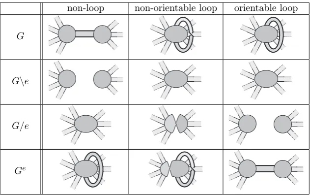
e∪u∪v as curves on G. For each resulting curve, attach a disc, which will form a vertex of G/e, by identifying its boundary component with the curve. Delete the interiors ofe, u and v from the resulting complex. We say thatG/eis obtained fromGbycontracting e. IfA⊆E,G/Adenotes the result of contracting all of the edges in A(the order in which they are contracted does not matter). A discussion about why this is the natural definition of contraction for ribbon graphs can be found in [18]. The local effect of contracting an edge of a ribbon graph is shown in Table 1. Note that contracting an edge inGmay change the number of vertices, number of components, or orientability. For instance, ifGis the orientable ribbon graph with one vertex and one edge, then contracting that edge results in the ribbon graph comprising two isolated vertices.
A ribbon graphH is aminor of a ribbon graphGifH is obtained fromGby a sequence of edge deletions, edge contractions, and deletions of isolated vertices. See Figure 1 for an example.
An edge in a ribbon graph is a bridge if its deletion increases the number of components of the ribbon graph. It is a loop if it is incident with only one vertex. A loop is a non-orientable loop if, together with its incident vertex, it is homeomorphic to a M¨obius band, otherwise it is an
orientable loop. Two cyclesC1 andC2in Gare said to beinterlaced if there is a vertexv such that V(C1)∩V(C2) ={v}, andC1andC2are met in the cyclic orderC1C2C1C2 when travelling round
the boundary of the vertexv. A loop isnon-trivialif it is interlaced with some cycle inG. Otherwise the loop istrivial.
Our interest here is in various notions of duality from topological graph theory. A slower exposition of the constructions here can be found in, for example, [14, 18]. We start with Chmutov’s partial duals of [13]. Let G be a ribbon graph and A ⊆ E(G). The partial dual GA of G is obtained as
non-loop non-orientable loop orientable loop
G
G\e
G/e
[image:7.595.140.456.85.283.2]Ge
Table 1: Operations on an edgee(highlighted in bold) of a ribbon graph
geometric dual of Gcan be defined byG∗:=GE(G).
Next we consider the Petrie dual (also known as the Petrial), G×, of G (see Wilson [35]). Let
Gbe a ribbon graph andA⊆E(G). Thepartial Petrial, Gτ(A), of Gis the ribbon graph obtained fromGby for each edgee∈A, choosing one of the two arcs (a, b) whereemeets a vertex, detaching
efrom the vertex along that arc giving two copies of the arc (a, b), then reattaching it but by gluing (a, b) to the arc (b, a), where the directions are reversed (Informally, this can be thought of as adding a half-twist to the edgee.) ThePetrie dual ofGisG×:=Gτ(E(G). We often writeGτ(e)forGτ({e}).
See Figure 1 for an example.
The partial dual and partial Petrial operations together gives rise to a group action on ribbon graphs and the concept of twisted duality from [16]. LetGbe a ribbon graph andA⊆E(G). In the context of twisted duality we will useGδ(A)to denote the partial dualGAofG. Letw=w
1w2· · ·wn
be a word in the alphabet {δ, τ}. Then we define Gw(A) := (· · ·((Gw1(A))w2(A)· · ·)wn(A). LetG:=
hδ, τ|δ2, τ2,(δτ)3i, which is just a presentation of the symmetric group of degree three. It was shown
in [16] thatGacts on the setX ={(G, A) :Ga ribbon graph, A⊆E(G)} byg(G, A) := (Gg(A), A)
forg∈G.
Now suppose Gis a ribbon graph,A, B⊆E(G), and g, h∈G. DefineGg(A)h(B):= Gg(A)h(B). We say that two ribbon graphs G and H are twisted duals if there exist A1, . . . , An ⊆ E(G) and
g1, . . . , gn ∈Gsuch thatH =Gg1(A1)g2(A2)···gn(An). Observe that,
1. ifA∩B=∅, then Gg(A)h(B)=Gh(B)g(A), 2. Gg(A)= (Gg(e))g(A\e), and
3. Gg1(A)=Gg2(A)ifg1=g2 in the grouphδ, τ|δ2, τ2,(δτ)3i.
We note that Wilson’s direct derivatives and opposite operators from [35] result from restricting twisted duality to the whole edge setE(G).
2.3
Delta-matroids from ribbon graphs
G. In terms of ribbon graphs, a tree can be characterised as a genus 0 ribbon graph with exactly one boundary component. Dropping the genus 0 requirement gives a quasi-tree: a quasi-tree is a ribbon graph with exactly one boundary component. Quasi-trees play the role of trees in ribbon graph theory, and replacing “tree” with “quasi-tree” in the definition of a cycle matroid results in a delta-matroid. Let Gbe a ribbon graph. Then the delta-matroid ofG isD(G) := (E,F) where F
consists of the edge sets of the spanning ribbon subgraphs ofGthat form a quasi-tree when restricted to each connected component ofG.
Example 2.2. LetGbe the ribbon graph of Figure 1(a). ThenD(G) has 20 feasible sets, 10 of which are {3,4,6}, {3,4,7}, {3,5,6}, {3,5,7}, {4,5,6}, {4,5,7}, {3,4,5,6,7}, {3,4,6,7,8}, {3,5,6,7,8},
{4,5,6,7,8}. The remaining 10 are obtained by taking the union of each of these with{1,2}. It can be checked thatD(G/{3,8}\{1}) =D(G)/{3,8}\{1} andD(G{1,6,7}) =D(G)∗ {1,6,7}.
Fundamental delta-matroid operations and ribbon graph operations are compatible with each other, as in the following theorem. Part 4 is from [14]; the others are from [7].
Theorem 2.3 ((Bouchet [7], Chun et al. [14])). Let G= (V, E)be a ribbon graph. Then
1. D(G)min=M(G)andD(G)max= (M(G∗))∗;
2. D(G) =M(G)if and only if Gis a plane ribbon graph;
3. D(G)is a binary delta-matroid;
4. D(GA) =D(G)∗A, in particularD(G∗) =D(G)∗;
5. D(G\e) =D(G)\eandD(G/e) =D(G)/e, for eache∈E.
The significance of Theorem 2.3, as we will see, is that it provides the means to move between ribbon graphs and delta-matroids, giving new insights into the structure of delta-matorids.
For notational simplicity in this paper we will take advantage of the following abuse of notation. For disconnected graphs, a standard abuse of notation is to say that T is a spanning tree of G if the components of T are spanning trees of the components of G. We will say that Qis a spanning quasi-tree of Gif the components of Q are spanning quasi-trees of the components ofG. Thus we can say that the feasible sets ofD(G) are the edge sets of the spanning quasi-trees ofG. This abuse should cause no confusion.
3
Twists of matroids
Twists provide a way to construct one delta-matroid from another. As the class of matroids is not closed under twists, but every matroid is a matroid, it provides a way to construct delta-matroids from delta-matroids. Twisting therefore gives a way to uncover the structure of delta-delta-matroids by translating results from the much better developed field of matroid theory. For this reason, the class of delta-matroids that arise as twists of matroids is an important one. In this section we examine the structure of this class of delta-matroids. In particular, we provide both an excluded minor characterisation, and a rough structure theorem for this class. Of particular interest here is the way that we are led to the results: we use ribbon graph theory to guide us. Our results provide support for the claim in this paper and in [14] that ribbon graphs are to delta-matroids what graphs are to matroids.
In order to understand the class of delta-matroids that are twists of matroids, we start by looking for the ribbon graph analogue of the class of delta-matroids that are twists of matroids. For this suppose that G= (V, E) is a ribbon graph with delta-matroid D =D(G). We wish to understand when D is the twist of a matroid, that is, we want to determine if D =M ∗A for some matroid
D∗B = D(G)∗B = D(GB), but, by Theorem 2.32, D(GB) is a matroid if and only if GB is a plane graph. So D is a twist of a matroid if and only if G is the partial dual of a plane graph. Thus to understand the class of delta-matroids that are twists of matroids we look towards the class of ribbon graphs that are partial duals of plane graphs. Fortunately, due to connections with knot theory (see [26]), this class of ribbon graphs has been fairly well studied with both a rough structure theorem and an excluded minor characterisation.
The following tells us that it makes sense to look for an excluded minor characterisation of twists of matroids.
Theorem 3.1. The class of delta-matroids that are twists of matroids is minor-closed.
Proof. We will show that, given a matroidM and a subsetAof E(M), ifD= (E,F) =M ∗A and
D0 is a minor ofD, thenD0 =M0∗A0 for some minorM0 of M and some subsetA0 ofE(M0). If
e /∈AthenD\e= (M∗A)\e= (M\e)∗AandD/e= (M∗A)/e= (M/e)∗A. On the other hand, ife∈AthenD\e= (M∗A)\e= (M/e)∗(A−e) andD/e= (M∗A)/e= (M\e)∗(A−e).
An excluded minor characterisation of partial duals of plane graphs appeared in [28]. It was shown there that a ribbon graph G is a partial dual of a plane graph if and only if it contains no
G0-,G1- or G2-minor, whereG0 is the non-orientable ribbon graph on one vertex and one edge;G1
is the orientable ribbon graph given by vertex set {1,2}, edge set {a, b, c} with the incident edges at each vertex having the cyclic order abc, with respect to some orientation of G1; and G2 is the orientable ribbon graph given by vertex set{1}, edge set{a, b, c}with the cyclic orderabcabcat the vertex. (The result in [28] was stated for the class of ribbon graphs that present link diagrams, but this coincides with the class of partial duals of plane graphs.)
For the delta-matroid analogue of the ribbon graph result set:
• X0:=D(G0) = ({a},{∅,{a}});
• X1:=D(G1) = ({a, b, c},{{a},{b},{c},{a, b, c}});
• X2:=D(G2) = ({a, b, c},{{a, b},{a, c},{b, c},∅}).
Note that every twist of X0 is isomorphic to X0 and that every twist of X1 or X2 is isomorphic to eitherX1 orX2. In particular,X1=X2∗.
Then translating the ribbon graph result into delta-matroids suggests thatX0,X1 andX2should form the set of excluded minors for the class of delta-matroids that are twists of matroids. Previously Duchamp [15] had shown, but not explicitly stated, thatX1andX2are the excluded minors for the
class of even delta-matroids that are twists of matroids.
Theorem 3.2 ((Duchamp [15])). A delta-matroid D = (E,F) is the twist of a matroid if and only if it does not have a minor isomorphic toX0,X1, orX2.
Proof. Take a matroidM and a subset A ofE(M). As |B| =r(M) for eachB ∈ B(M), we know that the sizes of the feasible sets ofM∗Awill have even parity ifr(M) andAhave the same parity, otherwise they will all have odd parity. ThusM∗Ais an even delta-matroid, andX0is obviously the unique excluded minor for the class of even delta-matroids. An application of [15, Propositions 1.1 and 1.5] then gives thatX0,X1,X2is the complete list of the excluded minors of twists of matroids.
We now look for a rough structure theorem for delta-matroids that are twists of matroids. Again we proceed constructively via ribbon graph theory, starting with a rough structure theorem for the class of ribbon graphs that are partial duals of plane graphs, translating it into the language of delta-matroids, then giving a proof of the delta-matroid result.
A vertex v of a ribbon graph G is a separating vertex if there are non-trivial ribbon subgraphs
P and QofGsuch that (V(G), E(G)) = (V(P)∪V(Q), E(P)∪E(Q)), and E(P)∩E(Q) =∅ and
Example 3.3. For the ribbon graph Gof Figure 1(a), v is a separating vertex with P and Qthe subgraphs induced by edges 1, . . . ,5 and by 6,7,8. G admits plane-biseparations. The edge sets
{1,6,7}, {2,6,7}, {2,3,4,5,8}, and {1,3,4,5,8} are exactly those that define plane-biseparations.
GA is plane if and only ifAis one of these four sets.
In [26], the following rough structure theorem was given:
Theorem 3.4 ((Moffatt [26])). LetG be a ribbon graph. Then the partial dualGA is a plane graph if and only if Adefines a plane-biseparation ofG.
Thus we need to translate a plane-biseparation into the language of delta-matorids. Since, by Theorem 2.3 a ribbon graph G is plane if and only if D = D(G) is a matroid, the requirement that G\A and G\Ac are plane translates to D\A and D\Ac being matroids. For the analogue of
separability we make the following definition. A delta-matroid is separable if its lower matroid is disconnected.
For a ribbon graphGand non-trivial ribbon subgraphsP andQofG, we writeG=PtQwhen
G=P∪QandP∩Q=∅. If there are non-trivial ribbon subgraphsP and QofGand a vertexv
ofGsuch that G=P∪Qand P∩Q={v}then we writeG=P ⊕Q. It was shown in [14] that if
Gis a ribbon graph, thenD(G) is separable if and only if there exist ribbon graphsG1 andG2such that G=G1tG2or G=G1⊕G2. Thus the condition that every vertex ofGthat is incident with both edges inA and edges inAc is a separating vertex ofGbecomes that A is separating inDmin.
So Theorem 3.4 may be translated to delta-matroids as follows.
Theorem 3.5. Let D be a delta-matroid andAa non-empty proper subset ofE(D). ThenD∗Ais a matroid if and only if the following two conditions hold:
1. A is separating inDmin, and
2. D\A andD\Ac are both matroids.
We need some preliminary results before we can prove this theorem. In the case that D is the twist of a matroid, we can describe the upper and lower matroids ofD precisely.
Lemma 3.6. Let M = (E,B) be a matroid and A be a subset of E. Let D = M ∗A. Then
Dmin=M/A⊕(M\Ac)∗.
Proof. Since we restrict our attention to the smallest sets of the formB4A, whereB ∈ B, we need only to consider those bases of M that share the largest intersection with A. That is, we think of building a basis forM by first finding a basis ofM\Ac and then extending that independent set to
a basis of M. Let IA be a basis of M\Ac and let BA be a basis of M such that IA ⊆BA. Then
A4BA= (BA−IA)∪(A−IA). Now,BA−IAis a basis inM/AandA−IAis the complement of a
basis inM\Ac, soB
A4Ais a basis ofM/A⊕(M\Ac)∗. Thus every basis ofDmincan be constructed
in this way. On the other hand, ifB0 is a basis of M/A⊕(M \Ac)∗, thenB0 =B1∪B2 where B1 is a basis ofM/AandB2is the complement of a basis of M\Ac. Thus B04A=B1∪(A−B2) is a basis ofM, soB0 is a feasible set ofD. As all bases ofM/A⊕(M\Ac)∗ are equicardinal and each basis ofDmin is a basis ofM/A⊕(M\Ac)∗,|B0|=r(Dmin), soB0 is a basis ofDmin.
Lemma 3.7. Let M = (E,B) be a matroid and let A be a subset of E. Let D = M ∗A. Then
Dmax=M \A⊕(M/Ac)∗.
Proof. As the feasible sets of (Dmax)∗ are just the feasible sets of (D∗)min, we deduce thatDmax=
((D∗)min)∗. Now (D∗)min= ((M∗A)∗E)min= ((M∗E)∗A)min= (M∗∗A)min. Lemma 3.6 implies
that (M∗∗A)
min=M∗/A⊕(M∗\Ac)∗. Then
M∗/A⊕(M∗\Ac)∗= (M\A)∗⊕((M/Ac)∗)∗= (M\A)∗⊕(M/Ac).
We deduce that (D∗)min = (M\A)∗⊕(M/Ac), thus ((D∗)min)∗ = ((M\A)∗⊕(M/Ac))∗. This last
The next two corollaries follow immediately from Lemma 3.6 and Lemma 3.7 and the fact that, for a given field F, the class of matroids representable over F is closed under taking minors, duals, and direct sums.
Corollary 3.8. Let C be a class of matroids that is closed under taking minors, duals, and direct sums. If M ∈ C andA⊆E(M), then(M∗A)min∈ C and(M∗A)max∈ C.
Corollary 3.9. Given a matroid M and subsetA of E(M), both (M ∗A)min and (M ∗A)max are
representable over any field that M is.
The proof of the following lemma can be found in [14].
Lemma 3.10. Let D= (E,F)be a delta-matroid, letA be a subset ofE and lets0= min{|B∩A|:
B∈ B(Dmin)}. Then for anyF∈ F we have |F∩A| ≥s0.
We can now prove Theorem 3.5.
of Theorem 3.5. Suppose first that M := D∗A is a matroid. Then D =M ∗A and Lemma 3.6 shows thatA is separating inDmin. The feasible sets ofD\Aare given by
F(D\A) ={F−A:F ∈ F(D), |F∩A| ≤ |F0∩A|for allF0∈ F(D)}.
So the feasible sets ofD\Aare obtained by deleting the elements inAfrom those feasible sets ofD
having smallest possible intersection withA. AsD=M∗A, we obtain
F(D\A) ={B∩Ac:B∈ B(M), |B∩A| ≥ |B0∩A|for allB0∈ B(M)}.
Because all bases ofM have the same number of elements, we see that all feasible sets ofD\Aalso have the same number of elements and consequentlyD\Ais a matroid. Similarly the feasible sets ofD\Ac form a matroid.
We now prove the converse. Letr=rDmin(A) andr
0=r
Dmin(A
c). We will show that any feasible
setF ofDsatisfies|F∩A| − |F∩Ac|=r−r0. This condition implies that all feasible sets ofD∗A
have the same size which is enough to deduce thatD∗Ais a matroid, as required.
Because A is separating in Dmin, any F0 in Fmin must satisfy |F0∩A| =r and|F0∩Ac|=r0.
Now Lemma 3.10 implies that any feasible setF ofD satisfies|F∩A| ≥r and|F∩Ac| ≥r0. We claim that a feasible setF satisfies|F∩A|=rif and only if|F∩Ac|=r0. The feasible sets ofD\A are given by
F(D\A) ={F−A:F∈ F(D), |F∩A|=r}.
Following condition 2, these sets form the bases of a matroid and consequently all have the same size, which must ber0. Therefore ifF is inF(D) and satisfies|F∩A|=r, then|F∩Ac|=r0. The converse is similar and so our claim is established.
We will now prove by induction on k that if F is a feasible set then|F∩A|=r+k if and only if|F∩Ac| =r0+k. We have already established the base case when k= 0. Suppose the claim is true for allk < l. IfF is a feasible set satisfying|F ∩A|=r+l, then using induction, we see that
|F∩Ac| ≥r0+l. Suppose then there is a feasible setF satisfying|F∩A|=r+land|F∩Ac|> r0+l. LetF1 be a member ofFmin. So|F1∩A|=rand|F1∩Ac|=r0. Now chooseF2 to be a feasible set
with|F2∩A|=r+l,|F2∩Ac|> r0+land|F2∩F1∩A|as large as possible amongst such sets. There exists x∈(F2−F1)∩A and clearly x∈F14F2. Hence there exists y belonging toF14F2 such thatF3=F24 {x, y} is feasible. Howevery is chosen, we must have|F3∩A|<|F3∩Ac|. Therefore
the inductive hypothesis ensures that|F3∩A| ≥ |F2∩A|and soy∈F1∩A. But thenF3 is a feasible
set ofD with|F3∩A|=r+l,|F3∩A0|> r0+l and|F3∩F1∩A|>|F2∩F1∩A|, contradicting the
We say that a ribbon graph Gis the join ofP andQ, written G=P∨Q, ifP and Qare two disjoint non-trivial ribbon graphs andG can be obtained by choosing an arc on the boundary of a vertex in P that does not intersect an edge, and doing likewise inQ, then identifying the two arcs. The two vertices that were identified become a single vertex ofG.
It is easily deduced from Proposition 5.22 of [14] that D(G) is disconnected if and only if there exist ribbon graphsG1 andG2 such thatG=G1tG2 orG=G1∨G2. In [26], it was shown thatG
andGAare both plane graphs if and only if we can writeG=H1∨ · · · ∨H
l, where eachHi is plane
andA=S
i∈IE(Hi), for some I⊆ {1, . . . , l}. This result extends to matroids as follows.
Theorem 3.11. Let M = (E,B)be a matroid and Abe a subset of E. Then M∗A is a matroid if and only ifA is separating orA∈ {∅, E}.
Proof. The minimum-sized sets and maximum-sized sets inB 4Ahave sizer(M)−r(A) +|A| −r(A) andr(E−A) +|A| −(r(M)−r(E−A)), respectively. The collectionB 4Ais the set of bases of a matroid if and only if they all have equal cardinality, or equivalently,
r(M)−r(A) +|A| −r(A) =r(E−A) +|A| −(r(M)−r(E−A)).
Simplifying yieldsr(M) =r(A) +r(E−A), which occurs if and only ifAis separating orA∈ {∅, E}, [30, Proposition 4.2.1],
We complete this section by generalizing a result of Welsh [33] regarding the connection between Eulerian and bipartite binary matroids. A graph is said to beEulerian if there is a closed walk that contains each of the edges of the graph exactly once, and a graph is bipartite if there is a partition (A, B) of the vertices such that no edge of the graph has both endpoints inAor both inB. Acircuit
in a matroid is a minimal dependent set and a cocircuit in a matroid is a minimal dependent set in its dual. A matroidM is said to beEulerian if there are disjoint circuitsC1, . . . , Cp in M such that
E(M) =C1∪ · · · ∪Cp. A matroid is said to bebipartite if every circuit has even cardinality.
A standard result in graph theory is that a plane graphGis Eulerian if and only ifG∗is bipartite. This result also holds for binary matroids.
Theorem 3.12((Welsh [33])). A binary matroid is Eulerian if and only if its dual is bipartite.
Once again, by considering delta-matroids as a generalization of ribbon graphs, we can determine when the twist of a binary bipartite or Eulerian matroid is either bipartite or Eulerian. In [23] it was shown that, ifGis a plane graph with edge setE andA⊆E, then
1. GA is bipartite if and only if the components ofG\Ac andG∗\A are Eulerian; 2. GA is Eulerian if and only ifG\Ac andG∗\Aare bipartite.
Recalling that, whenGis plane,D(G) is a matroid, and thatD(GA) =D(G)∗Asuggests an extension
of this result to twists of binary matroids, but first we need to introduce some terminology. The circuit spaceC(M) (respectively cocircuit space C∗(M)) of a binary matroid M = (E,B) comprises all subsets ofEwhich can be expressed as the disjoint union of circuits (respectively cocircuits). Both spaces include the empty set. It is not difficult to see that a subset ofE belongs to the circuit space (respectively cocircuit) space if and only if it has even intersection with every cocircuit (respectively circuit) [30]. The bicycle spaceBI(M) ofM is the intersection of the circuit and cocircuit spaces. It is not difficult to show that for any binary matroidM, we have C(M/A) ={C−A:C∈ C(M)}. FurthermoreC(M∗) =C∗(M) which implies thatBI(M) =BI(M∗).
Theorem 3.13. Let M = (E,B)be a binary matroid,A be a subset ofE andD=M∗A. 1. IfM is bipartite, thenDmin is bipartite if and only ifA∈ BI(M).
Proof. We prove the first part. Lemma 3.6 implies thatDmin=M/A⊕(M\Ac)∗. SoDminis bipartite exactly when bothM/Aand (M\Ac)∗ are bipartite. Every circuit of a matroid has even cardinality if and only if every element of its circuit space has even cardinality. Consequently every circuit of
M/A has even cardinality if and only if C−A has even cardinality for every C ∈ C(M). Because every circuit ofM has even cardinality, this occurs if and only ifC∩Ahas even cardinality for every
C∈ C(M), which corresponds toA∈ C∗(M).
On the other hand (M\Ac)∗=M∗/(E−A). This matroid is bipartite exactly when every element ofC(M∗) has an even number of elements not belonging to E−A. Equivalently the intersection of any circuit ofC(M∗) with Ahas even cardinality which occurs if and only ifA ∈ C∗(M∗) =C(M). SoDmin is bipartite if and only ifA∈ BI(M).
The proof of the second part is very similar and so is omitted.
Corollary 3.14. LetM = (E,B)be a binary matroid,A be a subset ofE andD=M∗A. 1. IfM is Eulerian, thenDmin is bipartite if and only ifE−A∈ BI(M);
2. IfM is bipartite, thenDmin is Eulerian if and only ifE−A∈ BI(M).
Proof. The first part follows from applying Theorem 3.13 toM∗and by using Theorem 3.12, because
M∗ is bipartite andD= (M∗)∗(E−A). The second part is similar.
4
Loop complementation and vf-safe delta-matroids
So far we have seen how the concepts of geometric and partial duality for ribbon graphs can serve as a guide for delta-matroid results on twists. In this section we continue to apply concepts of duality from topological graph theory to delta-matroid theory by examining the delta-matroid analogue of Petrie duality and partial Petriality.
Following Brijder and Hoogeboom [9], let D= (E,F) be a set system ande∈E. ThenD+eis defined to be the set system (E,F0) where
F0=F 4{F∪e:F∈ F ande /∈F}.
Ife1, e2∈E then (D+e1) +e2 = (D+e2) +e1. This means that ifA={e1, . . . , en} ⊆E we can
unambiguously define theloop complementationofD onA, byD+A:=D+e1+· · ·+en.
We remark that loop complementation is particularly natural in the context of binary delta-matroids. IfD=D(C) for some matrix C over GF(2), then formingD+ecoincides with changing the diagonal entry of C corresponding to e from zero to one or vice versa, and forming the delta-matroid of the resulting matrix. IfC is regarded as the adjacency matrix of a looped simple graph, then the loop complementation corresponds to adding or removing a loop at a vertex, explaining the name of the operation.
It is important to note that the set of delta-matroids is not closed under loop complementation. For example, let D = (E,F) with E={a, b, c} andF = 2{a,b,c}\ {a}. Then D is a delta-matroid, but D+a= (E,F0), whereF0 ={∅,{a},{b},{c},{b, c}}, is not a delta-matroid, since ifF1={b, c} andF2={a}, then there is no choice ofxsuch thatF14 {a, x} ∈ F0. To get around this issue, we often restrict our attention to a class of delta-matroids that is closed under loop complementation. A delta-matroid D = (E,F) is said to be vf-safe if the application of every sequence of twists and loop complementations results in a delta-matroid. (The operations arising from sequences of twists and loop complementations are called vertex-flips, since in the binary case they can be viewed as operations on the vertices of a graph. Vf-safe stands for vertex-flip-safe.) The class of vf-safe delta-matroids is known to be minor closed and strictly contains the class of binary delta-delta-matroids (see for example [11]). In particular, as ribbon graphic delta-matroids are binary (Theorem 2.33), it follows that ribbon-graphic delta-matroids are also vf-safe.
Theorem 4.1. Let Gbe a ribbon graph andA⊆E(G). ThenD(G) +A=D(Gτ(A)).
Proof. Without loss of generality we assume that G is connected. To prove the proposition it is enough to show thatD(G) +e=D(Gτ(e)). To do this we describe how the spanning quasi-trees of Gτ(e)are obtained from those ofG.
Suppose that the boundary of the edge e, when viewed as a disc, consists of the four arcs [a1, b1],
[b1, b2] =:β, [b2, a2], and [a2, a1] =:α, where{α, β}={e} ∩V(G) are the arcs which attache to its
incident vertices (or vertex). Let H be a spanning ribbon subgraph of G. Consider the boundary cycle or cycles ofH containing the pointsa1, a2, b1, b2. Ife∈E(H) then the boundary components of H\e can be obtained from those ofH by deleting the arcs [a1, b1] and [b2, a2], then adding arcs [a1, a2] and [b1, b2]. Similarly, the boundary components of Hτ(e) can be obtained from those ofH
by deleting the arcs [a1, b1] and [b2, a2], then adding arcs [a1, b2] and [a2, b1]. Each time the number of boundary components ofH\eorHτ(e)is computed in the argument below this procedure is used. To relate the spanning quasi-trees ofGandGτ(e)letH be a spanning ribbon subgraph ofGthat contains e. Consider the boundary components (or component) containing the pointsa1, a2, b1, b2. If there is one component then they are met in the ordera1, b1, b2, a2or a1, b2, a2, b1 when travelling around the unique boundary component of H starting froma1 and in a suitable direction. If there
are two components, then one contains a1 and b1, and the other contains a2 and b2. Recall that f(Q) denotes the number of boundary components of a ribbon graphQ. Comparing the number of boundary components ofH\e andHτ(e) with those of H, we see that if the points a
1, a2, b1, b2 are
met in the ordera1, b1, b2, a2, then we havef(H\e) =f(H) + 1 andf(Hτ(e)) =f(H). If the points
are met in the ordera1, b2, a2, b1 then f(H\e) =f(H) and f(Hτ(e)) =f(H) + 1. If the points are
on two boundary components thenf(H\e) =f(H)−1 andf(Hτ(e)) =f(H)−1. This means that
for some integerk, two off(H),f(H\e) andf(Hτ(e)) are equal tokand the other is equal tok+ 1.
Note thatf(H\e) =f(Hτ(e)\e).
From the discussion above we can derive the following. Suppose that H\e is not a spanning quasi-tree ofG. ThenH is a spanning quasi-tree ofGif and only ifHτ(e)is a spanning quasi-tree of
Gτ(e). Now suppose thatH\eis a spanning quasi-tree of G. Then either H is a spanning quasi-tree of G or Hτ(e) is a spanning quasi-tree of Gτ(e), but not both. Finally, let D(G) = (E,F), and recall that the feasible sets of D(G) (respectivelyD(Gτ(e))) are the edge sets of all of the spanning quasi-trees ofG(respectivelyGτ(e)). From the above, we see that feasible sets ofD(Gτ(e)) are given byF 4{F∪e:F ∈ F such thate /∈F}. It follows that D(G) +A=D(Gτ(A)), as required.
For use later, we record the following lemma. Its straightforward proof is omitted.
Lemma 4.2. Let e be an element of a vf-safe delta-matroid D = (E,F)and let A ⊆E−e. Then
(D+A)/e= (D/e) +A and(D+A)\e= (D\e) +A.
In [9] it was shown that twists, ∗, and loop complementation, +, give rise to an action of the symmetric group of degree three on set systems. IfS= (E,F) is a set system, andw=w1w2· · ·wn
is a word in the alphabet{∗,+}(note that∗ and + are being treated as formal symbols here), then (S)w:= (· · ·((S)w1(E))w2(E)· · ·)wn(E). (1)
With this, it was shown in [9] that the group S =h∗,+| ∗2,+2,(∗+)3iacts on the set of ordered
pairs X ={(S, A) : S a set system, A ⊆E(G)}. Let S = (E,F) be a set system, A, B ⊆E, and
g, h∈G. LetSg(A)h(B) := (Sg(A))h(B). Let D1= (E,F) andD2 be delta-matroids. We say that
D2 is a twisted dualofD1if there exist A1, . . . An ⊆E andg1, . . . , gn∈Ssuch that
D2=D1g1(A1)g2(A2)· · ·gn(An).
It was shown in [9] that the following hold.
2. Dg(A) = (Dg(e))g(A\e)
3. Dg1(A) =Dg2(A) ifg1=g2in the grouph∗,+| ∗2,+2,(∗+)3i.
We have already shown that geometric partial duality and twists as well as Petrie duals and loop complementations are compatible. So it should come as no surprise that twisted duality for ribbon graphs and for delta-matroids are compatible as well.
Theorem 4.3. LetG=hδ, τ |δ2, τ2,(δτ)3iandS=h∗,+| ∗2,+2,(∗+)3ibe two presentations of the
symmetric group S3; and letη :G→S be the homomorphism induced by η(δ) =∗, and η(τ) = +.
Then if Gis a ribbon graph,A1, . . . An⊆E(G), andg1, . . . , gn ∈Gthen
D(Gg1(A1)g2(A2)···gn(An)) =D(G)η(g1)(A1)η(g2)(A2)· · ·η(g
n)(An).
Proof. The result follows immediately from Theorem 2.34 and Theorem 4.1.
We now return to the topic of binary and Eulerian matroids as discussed at the end of Section 3. Brijder and Hoogeboom [12] obtained results of a different flavour on delta-matroids obtained from Eulerian or bipartite binary matroids. To describe them we need some additional notation. Let
D= (E,F) be a set system andAbe a subset ofE. Then thedual pivotonA, denoted byD¯∗A, is defined by
D¯∗A:= ((D∗A) +A)∗A.
From the discussion on twisted duality above, it follows thatD¯∗A= ((D+A)∗A) +A. We shall use this observation and other similar consequences of twisted duality several times in this section.
LetM = (E,F) be a binary matroid. Brijder and Hoogeboom [12] showed thatM is bipartite if and only if M+E is an even delta-matroid, and thatM is Eulerian if and only ifM¯∗E is an even delta-matroid. These results are interesting in the context of ribbon graphs. In [16] it was shown that an orientable ribbon graphGis bipartite if and only if its Petrie dualG×is orientable, although, unfortunately, the result was misstated. In particular, ifGis plane, thenM(G) is bipartite if and only ifM(G) +E(G) is even, which is the graphic restriction of the first part of Brijder and Hoogeboom’s result. The ribbon graph analogue of the second part is that a plane graphGis Eulerian if and only ifG∗×∗is orientable. This is indeed the case: Gis Eulerian if and only ifG∗ is bipartite if and only if (G∗)× is orientable if and only if ((G∗)×)∗ is orientable. However, the result does not extend to all Eulerian ribbon graphs, for example, consider the ribbon graph consisting of one vertex and two orientable non-trivial loops.
An edge e of a ribbon graph Gis a loop if and only if eis a loop of D(G)min. (A loop e may,
however, belong to feasible sets of D(G) other than those forming the bases of its lower matroid.) Loops in ribbon graphs can be classified into several types: orientable or non-orientable, trivial or non-trivial. The authors proved in [14] that the orientability and triviality of a loop ein a ribbon graphGis easily determined fromD(G). For instance an edgeeis a trivial orientable loop of a ribbon graph Gif and only ifeis a loop inD(G). This gives a way of classifying the loops ofD(G)min. It
turns out that this classification may be usefully extended to classify the loops of the lower matroid of any delta-matroid. This is yet another example of topological graph theory guiding the theory of delta-matroids. As this classification follows exactly the classification of loops in ribbon graphs we extend the nomenclature from ribbon graphs to arbitrary delta-matroids. The following definition is from [14].
Definition 4.4. LetD= (E,F) be a delta-matroid. Takee∈E. Then 1. eis a ribbon loopifeis a loop inDmin;
4. a non-orientable ribbon loop e is trivial if F4eis in F for every feasible set F ∈ F and is
non-trivial otherwise.
Notice that a trivial orientable ribbon loop of a delta-matroid D is exactly a loop ofD.
The following result is a slight reformulation of Theorem 5.5 from [10] and is the key to under-standing the different types of ribbon loops in a vf-safe delta-matroid. Following the notation of [12], we setdD:=r(Dmin).
Theorem 4.5 ((Brijder, and Hoogeboom [10])). Let D be a vf-safe delta-matroid and let e ∈ E. Then two of Dmin, (D∗e)min and (D¯∗e)min are isomorphic. If M1 is isomorphic to two matroids
in {Dmin,(D∗e)min,(D¯∗e)min} and M2 is isomorphic to the third thenM1 is formed by taking the
direct sum of M2/e and the one-element matroid comprising e as a loop. In particular two of dD,
dD∗e anddD¯∗e are equal to dand the third is equal to d+ 1, for some integerd. Finally eis a loop in precisely two ofDmin,(D∗e)min and(D¯∗e)min.
The next lemma shows that the behaviour of each type of ribbon loop in delta-matroids under the various notions of duality is exactly as predicted by the behaviour of the corresponding type of loop in ribbon graphs.
Lemma 4.6. Let D= (E,F)be a delta-matroid and let e∈E. Then 1. e is a coloop inD if and only if eis a loop in D∗e,
2. e is neither a coloop nor a ribbon loop in D if and only if eis a non-trivial orientable ribbon loop in D∗e.
If in addition D is vf-safe, then
3. a ribbon loopeis orientableif and only if eis a ribbon loop inD¯∗e, 4. a non-orientable ribbon loop is trivial if and only if eis a loop ofD+e.
Proof. Parts 1 and 4 are straightforward and Part 3 follows from Theorem 4.5. We prove Part 2, first proving the only if statement. Ase is not a ribbon loop inD, it is a ribbon loop in D∗e and is orientable because it is not a ribbon loop in (D∗e)∗e=D. By 1, it is non-trivial inD∗esince
eis not a coloop in D. Conversely, ife is a non-trivial orientable ribbon loop inD∗e, then ase is orientable it is not a ribbon loop in (D∗e)∗e=D. By 1, it is not a coloop inD.
A more thorough discussion of how twisting transforms the various types of ribbon loops can be found in [14].
In a ribbon graph partial Petriality changes the orientability of a loop. The following results describe the corresponding changes in delta-matroids.
Lemma 4.7. LetD= (E,F)be a vf-safe delta-matroid and lete∈E. Theneis a ribbon loop inD
if and only ife is a ribbon loop in D+e. Moreover a ribbon loop, e, is non-orientable in D if and only if it is orientable in D+e, and e is trivial inD if and only if it is trivial in D+e. Finally, e
is a coloop inD if and only ifeis a coloop of D+e.
Proof. The bases of (D+e)minare the same as those ofDmin. Ifeis a ribbon loop inDthen no basis
ofDmin containse, soeis a ribbon loop inD+e. The converse follows because (D+e) +e=D. Suppose that e is a non-orientable ribbon loop in D. Then e is a ribbon loop inD∗e. So by the first part of this lemma, eis a ribbon loop in both D+e and (D∗e) +e. By twisted duality the latter is equal to (D+e)¯∗e. Consequently, by Part 3 of Lemma 4.6, e is an orientable ribbon loop in D+e. Conversely if e is an orientable ribbon loop in D+e, then it is a ribbon loop in (D+e)¯∗e= (D∗e) +e. By the first part of this lemma,eis a ribbon loop in bothD andD∗eand so it must be a non-orientable ribbon loop inD.
Next, the statement concerning triviality follows from the definition of trivial loops and the fact that (D+e) +e=D. Finally, ifeis a coloop ofD, theneis in every feasible set ofD, soD=D+e
The next three lemmas are needed in Section 5. Each is stated, perhaps a little unnaturally, in terms of the dual of a vf-safe delta-matroidD, but this is exactly what is required later.
Lemma 4.8. Let ebe an element of a vf-safe delta-matroid, D. Then
1. e is a non-trivial orientable ribbon loop inD∗ if and only ifeis a non-trivial orientable ribbon loop in (D+e)∗;
2. e is a loop inD∗ if and only if eis a loop in (D+e)∗;
3. e is a coloop inD∗ if and only if eis a trivial non-orientable ribbon loop in(D+e)∗;
4. e is neither a ribbon loop nor a coloop in D∗ if and only if e is a non-trivial non-orientable ribbon loop in(D+e)∗.
Proof. Notice thatD∗= (D∗(E(D)−e))∗eand (D+e)∗= ((D∗(E(D)−e))∗e)¯∗e. Consequently (D+e)∗= (D∗)¯∗e.
It follows from Part 3 of Lemma 4.6 that ifeis an orientable ribbon loop ofD∗, then it is a ribbon loop of (D∗)¯∗e= (D+e)∗. Moreover, as ¯∗is involutary, it follows thateis an orientable ribbon loop ofD∗if and only if it is an orientable ribbon loop of (D+e)∗. Furthermore it follows from Part 1 of Lemma 4.6 and the last part of Lemma 4.7 thateis loop inD∗if and only ifeis a loop in (D+e)∗. This proves the first two parts.
Ifeis not a ribbon loop ofD∗, then it follows from Theorem 4.5 thatemust be a ribbon loop of (D∗)¯∗e= (D+e)∗. Moreover, by definition, emust be a non-orientable ribbon loop of (D+e)∗. On the other hand, ifeis a non-orientable ribbon loop of (D+e)∗ then, by definition and Theorem 4.5, it is not a ribbon loop of (D+e)∗¯∗e=D∗. Finally it is easily seen that Part 1 implies that e is a coloop inD∗ if and only ifeis a trivial non-orientable ribbon loop of (D+e)∗. This proves the last two parts.
The next lemma is straightforward and its proof is omitted.
Lemma 4.9. Let ebe an element of a vf-safe delta-matroid, D= (E,F)and letA⊆E−e. Then 1. e is a loop inD if and only ifeis a coloop in (D+A)∗;
2. e is a trivial non-orientable ribbon loop inD if and only if eis a coloop in(D+A+e)∗.
Lemma 4.10. Let ebe an element of a vf-safe delta-matroid,D.
1. Ifeis a non-trivial orientable ribbon loop in D∗ then(D∗\e)min= ((D+e)∗\e)min.
2. Ifeis neither a ribbon loop nor a coloop in D∗ then(D∗/e)min= ((D+e)∗\e)min.
3. Ifeis a non-trivial non-orientable ribbon loop inD∗ then (D∗\e)min= ((D+e)∗/e)min.
Proof. We show first that 1 holds. If e is a ribbon loop in D∗ then (D∗\e)min = (D∗)min. If e
is a non-trivial orientable loop in D∗, it follows from Theorem 4.5 and Part 3 of Lemma 4.6 that (D∗)min= (D∗¯∗e)min. Using twisted duality
(D∗¯∗e)min= (((((D∗(E(D)−e))∗e)∗e) +e)∗e)min= ((D+e)∗)min.
By Part 1 of Lemma 4.8,eis a non-trivial orientable ribbon loop in (D+e)∗ and so ((D+e)∗)min=
((D+e)∗\e)min.
Next, we show that 2 holds. If e is neither a ribbon loop nor a coloop inD∗, then by Part 4 of Lemma 4.8,eis a non-trivial non-orientable ribbon loop in (D+e)∗. Consequently ((D+e)∗\e)min=
((D+e)∗)min. Becauseeis non-orientable, it follows from Theorem 4.5 and Part 3 of Lemma 4.6 that
((D+e)∗)
min= (((D+e)∗)∗e)min and this can be shown to be equal to ((D∗∗e) +e)min. Because eis not a ribbon loop inD∗, the lower matroids ofD∗/eand (D∗∗e) +ecoincide.
We conclude our proof by showing that 3 holds. By Part 4 of Lemma 4.8 with D and D+e
interchanged, e is neither a ribbon loop nor a coloop of (D+e)∗. Applying 2 with D replaced by
D+e, we get ((D+e)∗/e)min= (((D+e) +e)∗\e)min or equivalently ((D+e)∗/e)min= (D∗\e)min
5
The Penrose and characteristic polynomials
The Penrose polynomial was defined implicitly by Penrose in [31] for plane graphs, and was extended to all ribbon graphs (equivalently, all embedded graphs) in [17]. The advantage of considering the Penrose polynomial of ribbon graphs, rather than just plane graphs, is that it reveals new properties of the Penrose polynomial (of both plane and non-plane graphs) that cannot be realised exclusively in terms of plane graphs. The (plane) Penrose polynomial has been defined in terms of bicycle spaces, left-right facial walks, or states of a medial graph. Here, as in [19], we define it in terms of partial Petrials.
LetGbe a ribbon graph. Then thePenrose polynomial,P(G;λ)∈Z[λ], is defined by
P(G;λ) := X
A⊆E(G)
(−1)|A|λf(Gτ(A)).
Recall, from Section 2.2, thatf(G) denotes the number of boundary components ofG.
The Penrose polynomial has been extended to both matroids and delta-matroids. In [2] Aigner and Mielke defined the Penrose polynomial of a binary matroidM = (E,F) as
P(M;λ) = X
X⊆E
(−1)|X|λdim(BM(X)), (2)
whereBM(X) is the binary vector space formed of the incidence vectors of the sets in the collection
{A∈ C(M) :A∩X ∈ C∗(M)}.
Brijder and Hoogeboom defined the Penrose polynomial in greater generality for vf-safe delta-matroids in [12]. Recall that ifD= (E,F) is a vf-safe delta-matroid, andX ⊆E, then thedual pivotonX is
D¯∗X := ((D∗X)+X)∗X, and thatdD:=r(Dmin). ThePenrose polynomialof a vf-safe delta-matroid
D is then
P(D;λ) := X
X⊆E
(−1)|X|λdD∗E¯∗X. (3)
It was shown in [12] that when the delta-matroidD is a binary matroid, Equations (2) and (3) agree. Furthermore, our next result shows that Penrose polynomials of matroids and delta-matroids are compatible with their ribbon graph counterparts.
Theorem 5.1. Let Gbe a ribbon graph andD(G)be its ribbon-graphic delta-matroid. Then
P(G;λ) =λk(G)P(D(G);λ).
Proof. LetAbe a subset ofE(G). We have
D(G)∗E¯∗A=D(G)∗E∗A+A∗A=D(Gδ(E)δ(A)τ(A)δ(A)) =D(Gδ(Ac)δ(A)δ(A)τ(A)δ(A)) =D(Gτ(A)δ(E)).
Then asD(Gτ(A)δ(E))min=M(Gτ(A)δ(E)), we have
r(D(Gτ(A)δ(E))min) =v(Gτ(A)δ(E))−k(Gτ(A)δ(E)) =f(Gτ(A))−k(G),
using that the number of vertices of a ribbon graph is equal to the number of boundary components of its dual. The equality of the two polynomials follows.
was shown that the Penrose polynomial of a ribbon graph admits such a relation. If Gis a ribbon graph, ande∈E(G), then
P(G;λ) =P(G/e;λ)−P(Gτ(e)/e;λ). (4) Recall that for a ribbon graphGand non-trivial ribbon subgraphsPandQofG, we writeG=PtQ
whenG is the disjoint union ofP and Q, that is, whenG=P ∪Qand P∩Q=∅. The preceding identity together with the multiplicativity of the Penrose polynomial,
P(G1tG2) =P(G1)·P(G2),
and its valueλon an isolated vertex provides a recursive definition of the Penrose polynomial. The Penrose polynomial of a vf-safe delta-matroid also admits a recursive definition.
Proposition 5.2 ((Brijder and Hoogeboom [12])). Let D = (E,F) be a vf-safe delta-matroid and
e∈E.
1. Ifeis a loop, then P(D;λ) = (λ−1)P(D/e;λ).
2. Ifeis a trivial non-orientable ribbon loop, then P(D;λ) =−(λ−1)P((D+e)/e;λ). 3. Ifeis not a trivial ribbon loop, thenP(D;λ) =P(D/e;λ)−P((D+e)/e;λ). 4. IfE=∅, then P(D;λ) = 1.
The recursion relation above for P(D) replaces (D¯∗e)\e for (D+e)/e in its statement in [12], but it is easy to see that (D+e)/eand (D¯∗e)\ehave exactly the same feasible sets. We have used (D+e)/erather than (D¯∗e)\eto highlight the compatability with Equation (4).
Observe that Equation (4) and a recursive definition for the ribbon graph version of the Penrose polynomial can be recovered as a special case of Proposition 5.2 via Theorem 5.1. It is worth noting that Equation (4) cannot be restricted to the class of plane graphs, and analogously that Proposition 5.2 cannot be restricted to binary matroids. Thus restricting the polynomial to either of these classes, as was historically done, limits the possibility of inductive proofs of many results. This further illustrates the advantages of the more general settings of ribbon graphs or delta-matroids.
Next, we show that the Penrose polynomial of a delta-matroid can be expressed in terms of the characteristic polynomials of associated matroids. The characteristic polynomial, χ(M;λ), of a matroidM = (E,B) is defined by
χ(M;λ) := X
A⊆E
(−1)|A|λr(M)−r(A).
The characteristic polynomial is known to satisfy deletion-contraction relations (see, for example, [34]).
Lemma 5.3. Let ebe an element of a matroid M.
1. Ifeis a loop, then χ(M;λ) = 0.
2. Ifeis a coloop, thenχ(M;λ) = (λ−1)χ(M/e;λ) = (λ−1)χ(M\e;λ). 3. Ifeis neither a loop nor a coloop, thenχ(M;λ) =χ(M\e;λ)−χ(M/e;λ).
We define thecharacteristic polynomial,χ(D;λ), of a delta-matroidDto beχ(Dmin;λ). WhenD
is a matroid,D=Dmin, so this definition is consistent with the definition above of the characteristic
polynomial of a matroid.
To keep the notation manageable, we define Dπ(A)to be (D+A)∗.
Theorem 5.4. Let D= (E,F)be a vf-safe delta-matroid. Then
P(D;λ) = X
A⊆E
Proof. Throughout the proof, we make frequent use of the fact that if e is an element of a delta-matroidD, then (D∗e)/e=D\eand (D∗e)\e=D/e. The proof proceeds by induction on the number of elements ofE. If E =∅ then both sides of Equation (5) are equal to 1. So assume that
E6=∅and lete∈E. We have
X
A⊆E
(−1)|A|χ(Dπ(A);λ) = X
A⊆E−e
(−1)|A|χ(Dπ(A);λ)− X
A⊆E−e
(−1)|A|χ(Dπ(A∪e);λ). (6)
Suppose that eis a loop ofD. Then by Lemmas 4.83 and 4.91, eis a coloop inDπ(A)and a trivial
non-orientable ribbon loop in Dπ(A∪e). So for each A⊆E−e, χ(Dπ(A∪e);λ) = 0 by Lemma 5.31,
and by Lemma 5.32
χ(Dπ(A);λ) = (λ−1)χ(((Dπ(A))min)/e;λ).
Since e is a coloop in Dπ(A), we have (Dπ(A))min/e = (Dπ(A)/e)
min = ((D+A)∗/e)min. Using
Lemma 4.2,
((D+A)∗/e)min= ((D\e+A)∗)min= ((D/e+A)∗)min= ((D/e)π(A))min,
where the penultimate equality holds because e is a loop in D and hence D\e = D/e. Therefore
χ(((Dπ(A))
min)/e;λ) =χ((D/e)π(A);λ). Hence
X
A⊆E
(−1)|A|χ(Dπ(A);λ) = (λ−1) X
A⊆E−e
(−1)|A|χ((D/e)π(A);λ).
Using induction and Proposition 5.21, this equals (λ−1)P(D/e;λ) =P(D;λ).
Next suppose thateis a trivial non-orientable ribbon loop ofD. Then by Lemmas 4.83 and 4.92,
eis a trivial non-orientable ribbon loop in Dπ(A) and a coloop inDπ(A∪e). So for each A⊆E−e,
using Lemma 5.32 and Lemma 4.2,
χ(Dπ(A∪e);λ) = (λ−1)χ(((Dπ(A∪e))min)/e;λ) = (λ−1)χ(((D+e)\e)π(A);λ)
= (λ−1)χ(((D+e)/e)π(A);λ),
where the last equality follows from the fact thateis a loop ofD+e. Furthermore,χ(Dπ(A);λ) = 0,
by Lemma 5.31. Hence
X
A⊆E
(−1)|A|χ(Dπ(A);λ) =−(λ−1) X
A⊆E−e
(−1)|A|χ(((D+e)/e)π(A);λ).
Using induction and Proposition 5.22, this equals−(λ−1)P((D+e)/e;λ) =P(D;λ).
We have covered the cases where e is a trivial ribbon loop inD. So now we assume that this is not the case. Using induction, Proposition 5.23, and Lemma 4.2 we have
P(D;λ) =P(D/e;λ)−P((D+e)/e;λ)
= X
A⊆E−e
(−1)|A|χ((D/e)π(A);λ)− X
A⊆E−e
(−1)|A|χ(((D+e)/e)π(A);λ).
We will show that for eachA⊆E−e
First, suppose that e is a loop in Dπ(A). Now by Lemma 4.2, (D/e) +A = (D+A)/e and ((D+e)/e) +A= (D+A+e)/e. Moreover,eis a coloop inD+Aand soD+A+e=D+A. Hence
χ((D/e)π(A);λ) =χ(((D+e)/e)π(A);λ) and χ(Dπ(A);λ) =χ(Dπ(A∪e);λ).
Therefore Equation (7) holds.
Second, suppose thateis a non-trivial orientable ribbon loop inDπ(A). Then by Lemma 4.81,eis
also a non-trivial orientable ribbon loop inDπ(A∪e). Soeis a ribbon loop of bothDπ(A)andDπ(A∪e).
Consequently χ(Dπ(A);λ) = χ(Dπ(A∪e);λ) = 0. On the other hand, by Lemma 4.2, (D/e)π(A) =
(Dπ(A))\e and ((D+e)/e)π(A) = (Dπ(A∪e))\e. Applying Lemma 4.101 with D replaced by D+A
shows thatχ(Dπ(A)\e;λ) =χ((D+e)π(A)\e;λ) and henceχ((D/e)π(A);λ) =χ(((D+e)/e)π(A);λ).
Therefore Equation (7) holds.
Third, suppose that eis neither a coloop nor a ribbon loop inDπ(A). Then by Lemma 4.84, eis a non-trivial non-orientable ribbon loop inDπ(A∪e). Thereforeχ(Dπ(A∪e);λ) = 0. By Lemma 5.33, we have
χ(Dπ(A);λ) =χ(((Dπ(A))min)\e;λ)−χ(((Dπ(A))min)/e;λ).
We have ((Dπ(A))
min)\e= ((Dπ(A))\e)min. Using Lemma 4.2 this is in turn equal to ((D/e)π(A))min.
Consequently χ(((Dπ(A))
min)\e;λ) = χ((D/e)π(A);λ). Because e is not a ribbon loop in Dπ(A),
((Dπ(A))
min)/e= ((Dπ(A))/e)min. By Lemma 4.102 this equals ((Dπ(A)+e)\e)minwhich by Lemma 4.2
equals (((D+e)/e)π(A))
min. Hence χ(((Dπ(A))min)/e;λ) = χ(((D+e)/e)π(A);λ) and Equation (7)
follows.
The final case is similar. Suppose that e is a non-trivial non-orientable ribbon loop inDπ(A).
Then by Lemma 4.84 applied toD+A+e, eis neither a coloop nor a ribbon loop inDπ(A∪e). We
have χ(Dπ(A);λ) = 0. By Lemma 5.33, we have
χ(Dπ(A∪e);λ) =χ(((Dπ(A∪e))min)\e;λ)−χ(((Dπ(A∪e))min)/e;λ).
We have ((Dπ(A∪e))min)\e = ((Dπ(A∪e))\e)min. Using Lemma 4.2 this is in turn equal to (((D+ e)/e)π(A))min. Consequentlyχ(((Dπ(A∪e))min)\e;λ) =χ(((D+e)/e)π(A);λ). Becauseeis not a ribbon
loop in Dπ(A∪e), ((Dπ(A∪e))min)/e = ((Dπ(A∪e))/e)min. By Lemma 4.103 this equals (Dπ(A)\e)min.
Using Lemma 4.2, this equals ((D/e)π(A))min. Henceχ(((Dπ(A∪e))min)/e;λ) =χ((D/e)π(A);λ) and
Equation (7) follows.
Therefore the result follows by induction.
If Gis a graph or ribbon graph andM(G) its cycle matroid, then χ(M(G);λ) =λ−k(G)χ(G;λ),
where theχon the right-hand side refers to the chromatic polynomial ofG. Combining this fact with Theorem 5.1 allows us to recover the following result as a special case of Theorem 5.4.
Corollary 5.5((Ellis-Monaghan and Moffatt [17, 19])). Let Gbe a ribbon graph. Then
P(G;λ) = X
A⊆E(G)
(−1)|A|χ((Gτ(A))∗;λ),
whereχ(H;λ) denotes the chromatic polynomial ofH.
In fact, in keeping with the spirit of this paper, it was the existence of this ribbon graph polynomial identity that led us to formulate Theorem 5.4.
We end this paper with some results regarding the transition polynomial. As observed by Jaeger in [24], the Penrose polynomial of a plane graph arises as a specialization of the transition polynomial,
LetEbe a set. We defineP3(E) :={(E1, E2, E3) :E =E1∪E2∪E3, Ei∩Ej=∅ for eachi6=j}.
That is,P3(E) is the set of ordered partitions of Einto three, possibly empty, blocks.
LetGbe a ribbon graph andRbe a commutative ring with unity. Aweight systemforG, denoted (α,β,γ), is a set of ordered triples of elements in R indexed by E =E(G). That is, (α,β,γ) :=
{(αe, βe, γe) :e∈E, andαe, βe, γe∈R}. Thetopological transition polynomial, Q(G,(α,β,γ), t)∈
R[t], is defined by
Q(G,(α,β,γ), t) := X
(A,B,C)∈P3(E(G))
Y
e∈A
αe
Y
e∈B
βe
Y
e∈C
γe
tf(Gτ(C)\B). (8)
If, in the set of ordered triples (α,β,γ), we have (αe, βe, γe) = (α, β, γ) for alle∈E(G), then we
write (α, β, γ) in place of (α,β,γ).
On the delta-matroid side, in [11] the transition polynomial of a vf-safe delta-matroid was intro-duced. SupposeD= (E,F) is a delta-matroid. A weight system (α,β,γ) forDis defined just as it was for ribbon graphs above. Then thetransition polynomialof a vf-safe delta-matroid is defined by
Q(α,β,γ)(D;t) =
X
(A,B,C)∈P3(E)
Y
e∈A
αe
Y
e∈B
βe
Y
e∈C
γe
tdD∗B¯∗C. (9)
Again we use the notation (α, β, γ) to denote the weight system in which each e ∈ E has weight (α, β, γ).
We will need a twisted duality relation for the transition polynomial. In order to state this relation, we introduce a little notation. Let (α,β,γ) = {(αe, βe, γe) : e∈E} be a weight system
for a delta-matroid D = (E,F), and let A ⊆ E. Define (α,β,γ)∗A to be the weight system
{(αe, βe, γe) :e∈E\A} ∪ {(βe, αe, γe) :e∈A}. Also define, (α,β,γ) +A to be the weight system
{(αe, βe, γe) :e∈E\A} ∪ {(αe, γe, βe) :e∈A}. For each wordw=w1. . . wn∈ h∗,+| ∗2,+2,(∗+)3i
define
(α,β,γ)w(A) := (α,β,γ)w1(A)w2(A)· · ·wn(A).
Theorem 5.6 ((Brijder and Hoogeboom [11])). Let D = (E,F) be a vf-safe delta-matroid. If
A1, . . . , An ⊆E, andg1, . . . , gn ∈ h∗,+| ∗2,+2,(∗+)3i, andΓ =g1(A1)g2(A2)· · ·gn(An), then
Q(α,β,γ)(D;t) =Q(α,β,γ)Γ((D)Γ;t).
Once again we see that a delta-matroid polynomial is compatible with a ribbon graph polynomial.
Proposition 5.7. Let G= (V, E) be a ribbon graph and D(G)be its ribbon-graphic delta-matroid. Then
Q(G; (α,β,γ), t) =tk(G)Q(β,α,γ)(D(G);t).
Proof. By Theorem 5.6, tk(G)Q(β,α,γ)(D(G);t) =tk(G)Q(α,β,γ)(D(G)∗E);t). Then, by comparing
Equation (8) and Equation (9) we see that to prove the theorem it is to sufficient to prove that
dD(G)∗E∗B¯∗C+k(G) =f(Gτ(C)\B) for all disjoint subsetsB andC of E(G). Theorem 4.3 and the
properties of twisted duals from Section 4 give
D(G)∗E∗B¯∗C=D(Gδ(E)δ(B)δτ δ(C)) =D(Gδ(A)τ δ(C)),
whereA=E−(B∪C). Then using thatr(D(G)min) =v(G)−k(G), the properties of twisted duals
once again and that contracting an edge from a ribbon graph does not change its number of boundary components
dD(G)∗E∗B¯∗C=r((D(G)∗E∗B¯∗C)min) =r(D(Gδ(A)τ δ(C))min)
=v(Gδ(A)τ δ(C))−k(Gδ(A)τ δ(C)) =f(Gδ(A)τ δ(C)δ(E))−k(G)
=f(Gτ(C)δ(B))−k(G) =f(Gτ(C)δ(B)/B)−k(G) =f(Gτ(C)\B)−k(G),