SARALEES NADARAJAH AND SAMUEL KOTZ
Received 11 October 2004
A generalized logistic distribution is proposed, based on the fact that the difference of two independent Gumbel-distributed random variables has the standard logistic distribution.
1. Introduction
IfX1 andX2 are independent Gumbel-distributed random variables with the common
cdf
F(x)=exp−exp(−x), (1.1)
then it is well known that the differenceZ=X1−X2has the standard logistic distribution
with the pdf
fZ(z)= exp(z)
1 + exp(z)2 (1.2)
for−∞< z <∞. The properties of this distribution and its generalizations have been studied by several authors. Of particular eminence are the numerous papers on this topic by Professor N. Balakrishnan and his colleagues; see, for example, Balakrishnan [1,2,3], Balakrishnan and Aggarwala [4], Balakrishnan et al. [5,7,12], Balakrishnan and Chan [6], Balakrishnan and Joshi [8], Balakrishnan and Kocherlakota [9], Balakrishnan and Leung [10], Balakrishnan and Malik [11], Balakrishnan and Puthenpura [13], Balakrish-nan and Sandhu [14], and BalakrishBalakrish-nan and Wong [15].
In this short note, we construct a new generalization of (1.2) by takingXi,i=1, 2, to have the general Gumbel distribution with the cdf
Fi(x)=exp
−exp
−x−µi σi
(1.3)
for−∞< x <∞,−∞< µi<∞, andσi>0. This distribution (which is also known as the extreme-value distribution of type I) has received special attention in the probabilistic-statistical literature and in various applications in the second half of the twentieth century.
Copyright©2005 Hindawi Publishing Corporation
A recent book by Kotz and Nadarajah [16], which describes this distribution, lists over fifty applications ranging from accelerated life testing through to earthquakes, floods, horse racing, rainfall, queues in supermarkets, sea currents, wind speeds, and track race records (to mention just a few).
2. The generalization
The pdf corresponding to (1.3) is
fi(x)=σ1 i
exp
−x−µi σi exp −exp
−x−µi σi
, (2.1)
and thus the pdf ofZ=X1−X2can be written as
fZ(z)= ∞
−∞f1(x)f2(x−z)dx
= 1
σ1σ2
∞
−∞exp
−x−µ1
σ1 exp −exp
−x−µ1
σ1
×exp
−x−z−µ2
σ2 exp −exp
−x−z−µ2
σ2
dx.
(2.2)
Settingy=exp(−x/σ1), (2.2) can be expressed as
fZ(z)= 1 σ2exp
µ1
σ1+
µ2+z
σ2
Iµ1,µ2,σ1,σ2 , (2.3)
whereIdenotes the integral
Iµ1,µ2,σ1,σ2 =
∞
0 y
σ1/σ2exp − exp µ1 σ1 y+ exp
µ2+z
σ2
yσ1/σ2
dy. (2.4)
We refer to (2.3) as thegeneralized logisticdistribution. The integral term in (2.4) is dif-ficult to calculate. However, for some particular choices of (µ1,µ2,σ1,σ2), one can obtain
the following explicit expressions.
(i) Ifσ1=σ2=σ, then by standard integration one can obtain
I= 1
expµ1/σ + exp
µ2+z /σ
2. (2.5)
If, in addition,µ1=µ2=µ, then the above reduces to
I=exp(−2µ/σ)
(ii) Ifσ1=2σ2, then one can show by [17, equation (2.3.15.7)] that
I=α √ πα 8 exp αβ2 4 2 erfc √ αβ 2
+αβ2erfc √
αβ 2
−α2β
4 , (2.7)
whereα=exp{(µ2+z)/σ2},β=exp{µ1/(2σ2)}, and erfc(·), denotes the complementary
error function defined by
erfc(x)=1−√2 π
x
0 exp
−t2 dt. (2.8)
(iii) If 0< σ1/σ2=p/q <1 (wherep≥1 andq≥1 are co-prime integers), then one can
show by [17, equation (2.3.1.13)] that
I=
q−1
j=0
(−α)j j! Γ
1 +p(1 +j) q
β−(1+p(1+j)/q)
×p+1Fq
1,∆
p, 1 + p(1 +j) q
;∆(q, 1 +j);(−1)qppαq qqβp
,
(2.9)
whereα=exp{(µ2+z)/σ2},β=exp(µ1/σ1),∆(k,a) denotes the sequence
∆(k,a)=a
k, a+ 1
k ,...,
a+k−1
k , (2.10)
mFndenotes the generalized hypergeometric function defined by
mFn
α1,...,αm;β1,...,βn;x =
∞
k=0
α1 k···
αm k
β1 k···
βn k
xk
k!, (2.11)
and (c)k=c(c+ 1)···(c+k−1) denotes the ascending factorial.
(iv) Ifσ1/σ2=p/q >1 (where p≥1 andq≥1 are coprime integers), then one can
show again by [17, equation (2.3.1.13)]that
I=
p−1
j=0
q(−β)j p j! Γ
1 +q(1 +j) p
α−(1+q(1+j)/ p)
×q+1Fp
1,∆
q, 1 +q(1 +j) p
;∆(p, 1 +j);(−1)pqqβp ppαq
,
(2.12)
0.3
0.2
0.1
0
f
(
x
)
−3 −2 −1 0 1 2 3
x
σ1/σ2=0.2
σ1/σ2=1
σ1/σ2=2
σ1/σ2=5
[image:4.468.144.325.67.269.2]σ1/σ2=10
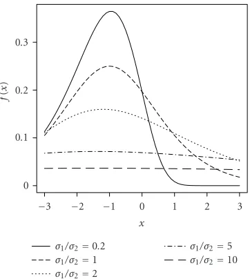
Figure 2.1. The generalized logistic pdf (2.3) forσ1/σ2=0.2, 1, 2, 5, 10,σ2=1,µ1=0, andµ2=1.
0.25
0.2
0.15
0.1
0.05
0
f
(
x
)
−3 −2 −1 0 1 2 3
x
σ1/σ2=0.2
σ1/σ2=1
σ1/σ2=2
σ1/σ2=5
[image:4.468.141.327.310.508.2]σ1/σ2=10
Figure 2.2. The generalized logistic pdf (2.3) forσ1/σ2=0.2, 1, 2, 5, 10,σ2=1,µ1=1, andµ2=0.
Figures2.1 and2.2 illustrate possible shapes of the pdf (2.3) for selected values of (µ1,µ2,σ1,σ2). The magnitude ofσ1/σ2 clearly controls the shape of the pdf. In fact, if
µ1=0, then
fZ(z)−→σ1
2
exp
µ2+z
σ2
exp
−exp
µ2+z
σ2
as σ1/σ2→0. Also, f(z)→0 for everyz∈(0,∞) as σ1/σ2→ ∞. On the other hand, if
µ1=0, thenf(z)→0 for everyz∈(0,∞) irrespective of whetherσ1/σ2→0 orσ1/σ2→ ∞.
3. Applications
The standard logistic distribution given by (1.2) has important uses in describing growth and as a substitute for the normal distribution. It has also attracted interesting applica-tions in the modeling of the dependence of chronic obstructive respiratory disease preva-lence on smoking and age, degrees of pneumoconiosis in coal miners, geological issues, hemolytic uremic syndrome data for children, physiochemical phenomenon, psycholog-ical issues, survival time of diagnosed leukemia patients, and weight gain data. The main feature of the generalized logistic distribution in (2.3) is that new parameters are intro-duced to control both location and scale. Thus, (2.3) allows for a greater degree of flexi-bility and we can expect this to be useful in many more practical situations.
References
[1] N. Balakrishnan,Order statistics from the half logistic distribution, J. Statist. Comput. Simulation 20(1985), no. 4, 287–309.
[2] ,Approximate maximum likelihood estimation for a generalized logistic distribution, J. Statist. Plann. Inference26(1990), no. 2, 221–236.
[3] N. Balakrishnan (ed.),Handbook of the Logistic Distribution, Statistics: Textbooks and Mono-graphs, vol. 123, Marcel Dekker, New York, 1992.
[4] N. Balakrishnan and R. Aggarwala,Relationships for moments of order statistics from the right-truncated generalized half logistic distribution, Ann. Inst. Statist. Math.48(1996), no. 3, 519–534.
[5] N. Balakrishnan, M. Ahsanullah, and P. S. Chan,On the logistic record values and associated inference, J. Appl. Statist. Sci.2(1995), no. 3, 233–248.
[6] N. Balakrishnan and P. S. Chan,Estimation for the scaled half logistic distribution under type II censoring, Comput. Statist. Data Anal.13(1992), no. 2, 123–141.
[7] N. Balakrishnan, S. S. Gupta, and S. Panchapakesan,Estimation of the mean and standard de-viation of the logistic distribution based on multiply type-II censored samples, Statistics27 (1995), no. 1-2, 127–142.
[8] N. Balakrishnan and P. C. Joshi,Means, variances and covariances of order statistics from sym-metrically truncated logistic distribution, J. Statist. Res.17(1983), no. 1-2, 51–61.
[9] N. Balakrishnan and S. Kocherlakota,On the moments of order statistics from the doubly trun-cated logistic distribution, J. Statist. Plann. Inference13(1986), no. 1, 117–129.
[10] N. Balakrishnan and M. Y. Leung,Means, variances and covariances of order statistics, BLUEs for the type I generalized logistic distribution, and some applications, Comm. Statist. Simulation Comput.17(1988), no. 1, 51–84.
[11] N. Balakrishnan and H. J. Malik,Moments of order statistics from truncated log-logistic distribu-tion, J. Statist. Plann. Inference17(1987), no. 2, 251–267.
[12] N. Balakrishnan, H. J. Malik, and S. Puthenpura,Best linear unbiased estimation of location and scale parameters of the log-logistic distribution, Comm. Statist. Theory Methods16(1987), no. 12, 3477–3495.
[14] N. Balakrishnan and R. A. Sandhu,Recurrence relations for single and product moments of order statistics from a generalized half logistic distribution with applications to inference, J. Statist. Comput. Simulation52(1995), no. 4, 385–398.
[15] N. Balakrishnan and K. H. T. Wong,Best linear unbiased estimation of location and scale pa-rameters of the half-logistic distribution based on typeIIcensored samples, Amer. J. Math. Management Sci.14(1994), no. 1-2, 53–101.
[16] S. Kotz and S. Nadarajah,Extreme Value Distributions. Theory and Applications, Imperial Col-lege Press, London, 2000.
[17] A. P. Prudnikov, Yu. A. Brychkov, and O. I. Marichev,Integrals and Series. Vol. 1. Elementary Functions, Gordon & Breach Science, New York, 1986.
[18] ,Integrals and Series. Vol. 2. Special Functions, Gordon & Breach Science, New York, 1988.
[19] ,Integrals and Series. Vol. 3. More Special Functions, Gordon & Breach Science, New York, 1990.
Saralees Nadarajah: Department of Statistics, University of Nebraska, Lincoln, NE 68583, USA
E-mail address:[email protected]
Samuel Kotz: Department of Engineering Management and Systems Engineering, The George Washington University, Washington, DC 20052, USA