APPLICATION OF NORMAL PROBABILITY DISTRIBUTION IN
ESTIMATING ANNUAL MAXIMUM AND MINIMUM TEMPERATURE IN THE
CONTEXT OF ASSAM
Dhritikesh Chakrabarty and Mahananda Gohain Department of Statistics Department of Statistics
Handique Girls’ College Purbanchal College,. Silapathar Guwahati – 781001, Assam, India Silapathar, Dhemaji – 787059, Assam, India
ABSTRACT
The normal probability distribution, also known as Gaussian distribution, was
discovered by a German mathematician Carl Friedrich Gauss in the year 1809. Some
authors credit this discovery to a French mathematician Abraham De Moivre who published
a paper in 1738 that showed the normal distribution as an approximation to the binomial
distribution discovered by James Bernoulli. The normal probability distribution plays the key
role not only in the development of most of the theories in statistics but also in the analysis of
data associated to many real phenomena. There are innumerable phenomena where one can
think of applying the theory of normal probability distribution to analyze the phenomena
based on data collected from them. In the case of temperature at a location, it is a reality that
temperature is a variable which changes continuously over time.. The temperature at a
location corresponds, in a year, to one maximum value and one minimum value that ought to
be constants if the pattern of this change is not influenced by some unnatural factor/factors.
There is scope of applying the theory of normal probability distribution in estimating the
annual maximum and minimum temperature at a location. In this study a method of has been
framed of for estimating the annual maximum and minimum temperature at a location by the
application of the area property of normal probability distribution. The method has been
applied in estimating the annual maximum and minimum of temperature in the context of
Assam.
Key Words:
Normal probability distribution, temperature, maximum, minimum, probabilistic estimation.
The normal probability distribution, also known as Gaussian distribution, was
discovered by a
German mathematician Carl Friedrich Gauss 1in the year 1809. Some authors credit this
discovery to
a French mathematician Abraham De Moivre2 who published a paper in 1738 that showed
the normal
distribution as an approximation to the binomial distribution discovered by James Bernoulli
(Bernoulli 3 , Chakrabarty 4-6, De Moivre 2,7 , Kendall and Stuart 8 , Walker and Lev 9 ,
Walker 10 ,
Brye 11, Hazewinkel 12 , Marsagilia 13 , Stigler 14 , Weisstein 15 et al). The normal
probability
distribution plays the key role in the theory of statistics as well as in the application of
statistics. There are innumerable situations (and / or problems) where one can think of
applying the theory of normal probability distribution to handle the situations (and / or to
search for their solutions).
The components of the climate (for example, average temperature, maximum temperature,
minimum temperature, humidity etc.) at a location/region have been changing continuously
over time. The change in a component occurs basically due to the following two
broad causes:
1. Assignable or controllable cause (or causes).
2. Chance cause.
The change in a component will be significant or equivalently effective or
equivalently
countable if and only if it occurs due to both the causes. On the other hand, the change in the
component will be insignificant or equivalently ineffective or equivalently negligible if and
only if it
occurs due to chance cause only. There is necessity of determining whether the change occurs
due to
both the causes or due to the chance cause only because, the task of controlling the change
arises only when the change occurs due to assignable cause (or causes). The temperature in a
location corresponds, in one year, to one maximum value and one minimum value that ought
There is necessity of a study on the natural maximum and of the natural minimum of
temperature. Chakrabarty 4-6 made a study on mean temperature, maximum temperature and
minimum temperature in respect of forecasting. In this study, attempt has also been made to
determine the natural maximum temperature and the natural minimum temperature in the
context of Assam. Here, a study has been made to search for some method of determining the
natural maximum and the natural minimum of temperature at a location by the application of
the area property of normal probability distribution. The method has been applied in
determining the natural maximum and the natural minimum of temperature in the context of
Assam. Once the values of the natural maximum temperature and the natural minimum
temperature in a location are known, it would be possible to know if the temperature of the
location has been influenced by some unnatural factor/factors by analyzing the past and
present scenario in respect of the temperature of the location.
2. GAUSSIAN DISCOVERY
The probability density function of the Normal Probability Distribution discovered by Gauss is described by the probability density function
f(x : μ , σ) = { σ (2ᴨ) ½}‒1. exp [ ‒ ½ {(x ‒ μ)/σ}2] ,
(2.1)
‒ ∞ < x < ∞ , ‒ ∞ < μ < ∞ , 0 < σ < ∞ .
Here, (i) X is the associated normal variable,
(ii) μ & σ are the two parameters of the distribution
And (iii) mean of X = μ & standard deviation of X = σ.
Note: If μ = 0 & σ = 1,
the density is standardized and X then becomes a standard normal variable.
Area Property of Normal Distribution
If X ~ N (μ , σ), then
(i) P(μ ‒ 1.96 σ < X < μ ‒ 1.96 σ) = 0.95,
(2.2)
(ii) P(μ ‒ 2.58 σ < X < μ ‒ 2.58 σ) = 0.99
(2.3)
& (iii) P( μ ‒ 3 σ < X < μ ‒ 3 σ) = 0.9973 .
(2.4)
(i) P(‒ 1.96 < X < 1.96) = 0.95,
(2.5)
(ii) P(‒ 2.58 < X < 2.58) = 0.99
(2.6)
& (iii) P(‒ 3 < X < 3) = 0.9973 .
(2.7)
3. METHOD OF DETERMINATION OF NATURAL EXTREMA OF TEMPERATURE
Let Y be the annual extremum (that is maximum or minimum) of temperature at a
location and Yi (i = 1, 2 , 3 , ………….. ) be the observation s on the annual extremum
temperature observed at a
location in the year i. The true/actual value of Y is unique, say μ(Y). But the observed values
are different which should be equal to μ(Y).
The variation in the observed values occur due to two types of causes/errors
namely+
1. Assignable Cause(s) that is (are) avoidable / controllable
And 2. Chance Cause/Error that is unavoidable / uncontrollable
The values of Yi should be constant if there exists no cause of variation in Yi over
years. However, chance cause (random cause) of variation exists always. Thus if no
assignable cause of variation exists in Yi over year, we have
Yi = μ(Y) + εi
(3.1)
where μ(Y) = the true value of Yi at the location in the year i
& εi = the amount of chance error associated to Yi(i = 1, 2 , 3 , …………..).
The variable Y, in this case, satisfies the mathematical model
Y = μ(Y) + ε
(3.2)
where μ(Y) = the true value of Y
& εi = the variable representing the chance error associated to Y.
It is to be noted that
(2) μ(Y) , ε1 , ε2 , ………… , εn are unknown.
& (3) the number of linear equations in (3.1) is n with n + 1 unknowns
implying that the equations are not solvable mathematically.
Following assumptions, which are reasonable, are made on the error component εi :
(1) ε1 , ε2 , ……….. , εn are unknown values of the variables ε.
(2) The values ε1 , ε2 , ………… , εn are very small relative to the respective values
X1 , X2 , ………… , Xn.
(3) The variable ε assumes both positive and negative values.
(4) P( ‒ a ‒ da < ε < ‒ a) = P( a < ε < a + da) for every real a.
(5) P( a < ε < a + da) > P( b < ε < b + db)
& P( ‒ a ‒ da < ε < ‒ a) < P( ‒ b ‒ db < ε < ‒ b)
for every real positive a < b.
(6) The facts (3), (4) & (5) together imply that ε obeys the normal probability law.
(7) Sum of all possible values of each ε is 0 (zero) which together with the fact (6)
implies that E(ε) = 0.
(8) Standard deviation of ε is unknown and small, say σε.
(9) The facts (6), (7) & (8) together imply that ε obeys the normal probability law
with mean (expectation) 0 &standard deviation σε. Thus
ε ~ N(0 , σε)
Now, under the assumption number (9),
Y ‒ μ ~ N (0 , σε) or equivalently Y ~ N(μ , σε) .
Also by the area property mentioned above,
(i) P (μ ‒ 1.96 σε < Y < μ ‒ 1.96 σε) = 0.95,
(3.2)
(ii) P (μ ‒ 2.58 σε < Y < μ ‒ 2.58 σε) = 0.99
(3.3)
& (iii) P (μ ‒ 3.00 σε < Y < μ ‒ 3.00 σε) = 0.9973 .
(3.4)
(iii) means that out of 10000 observations, maximum 27 observations fall outside the interval
(μ ‒ 3.00 σε , μ + 3.00 σε)
i.e. out of 100 observations maximum one observation will fall outside the interval
provided the
change in Y does not occur due to any assignable cause but occurs due to chance cause only
or
equivalently the change in Y is not significant. This principle/method can be applied to
determine whether the change in Y over year is significant.
Note The set of observations
Y1 , Y2 , ………,Yi , …….. , Yn
Constitute the population for the period from the year ‘1’ to the year ‘n’.
Thus, μ = Arithmetic Mean of(Y1 ,Y2 , ………, Yi, …….. , Yn)
(3.6)
and σε2= Variance of (Y1 , Y2 , ……, Yi, ….. , Yn)
(3.7)
Again due to the same logic, the intervals
(i) (μ ‒ 1.96 σε , μ + 1.96 σε) ,
(3.8)
(ii) (μ ‒ 2.58 σε , μ + 2.58 σε)
(3.9)
& (iii) ( ‒ 3.00 σε , μ + 3.00 σε)
(3.10)
are respectively 95% , 99% & 99.73% confidence intervals of Y.
Now, P{(Yi ‒ μ) / σε < 3} = 0.9973
implies that a random value of Y goes outside the interval
μ ‒ 3σε < Y i < μ + 3σε
(3.11)
is 0.0027 which is very small. This means, it is near certain that Y falls inside the interval
which in
other words means that it is natural that Y falls inside the interval. For this reason, this
interval is
termed as the natural interval of Y (Shewhart16, Grant17).
Thus in order to determine the natural interval (more specifically natural maximum and
minimum) of Y, it is required to determine μ and σε which can be obtained by applying the
relation (3.7) and (3.7) respectively.
4. DETERMINATION OF NATURAL EXTREMA OF TEMPERATURE IN THE CONTEXT
OF ASSAM
The objectives in the study are
(1) to investigate whether the changes in temperature, in Assam, that are occurred is
due to some unnatural cause or causes
and (2) to determine the natural maximum and the natural minimum of Temperature in the
context of
Assam.
To achieve the objectives, data on
(1) the maximum temperature
and (2) the minimum temperature at the locations covering Assam are needed.
Indian Meteorological Department has 41 locations (called stations in meteorological
terminology),
out of which 5 locations are situated in Assam more or less covering the state which are
Dibrugarh,
Dhubri, Guwahati, Tezpur and Silchar.
In the collection of data from these stations we had been supplied the prior information that
the
daily data suffer from inconsistency (undetectable and immeasurable) while monthly data are
almost
free from it. For this reasons, the raw data have been converted to monthly data. Thus, the
classified
data deals with
(1) the highest maximum temperature occurred in month i.e. monthly maximum
temperature
and (2) the lowest minimum temperature occurred in monthly i.e. monthly mimimum
temperature.
5. ANALYSIS OF DATA (Computations)
Step – 5.1: In the first step,
(1) the highest maximum temperature
and (2) the lowest minimum temperature
occurred in each of the 12 months at each of the 5 stations have been identified and collected.
Thus,
the collected data deal with
(1) the monthly maximum temperature
and (2) the monthly minimum temperature
for each of the 5 stations.
Step – 5.2: In the second step,
(1) the highest maximum temperature
and (2) the lowest minimum temperature
occurred in each year of each of the 5 stations have been identified. Thus, the identified data
deal with
(1) the annual maximum temperature
and (2) the annual minimum temperature
for each of the 5 stations.
Step – 5.3: In the third step, the two parameters namely mean μ and standard deviation σε have been
estimated for each of the characteristics
(1) the annual maximum temperature
and (2) the annual minimum temperature
for each of the 5 stations.
The parameters μ and σε for a specified station are nothing but the population mean and
population variance respectively of the specified characteristic. Thus the estimates of μ and σε
obtained are nothing but the estimates of the corresponding characteristics and the estimates
of the standard deviations of the corresponding estimates. The estimated values of annual
maximum temperature and annual minimum temperature with the respective estimated values
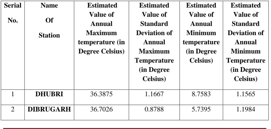
of the corresponding standard deviation have been presented in Table – 6.1.
Step – 5.4: In the next step, 95 % confidence interval of the two characteristics mentioned in
5.3 for each of the 5 stations have been computed. The values of them have been presented in
Table–6.2.
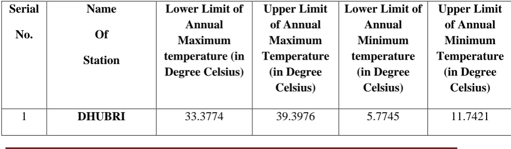
Step – 5.5: In the next step, 99 % confidence interval of the two characteristics ment ioned in
Step -5.3 for each of the 5 stations have been computed. The values of them have been presented in Table–6.3.
Step – 5.6: In the next step, natural interval of the two characteristics mentioned in Step – 5.3
for
each of the 5 stations have been computed. The values of them have been presented in Table – 6.4.
Step – 5.7: In the next step, it has been examined whether the observed values of each of the two
characteristics
(1) the annual maximum temperature
and (2) the annual minimum temperature
for each of the 5 stations lie within the corresponding interval obtained in Step – 5.6. The findings
have been presented in Table – 6.5
6. PRESENTATION OF RESULTS
Table – 6.1
(Mean of Annual Maximum Temperature and Annual Minimum Temperature with Standard Deviation) Serial No. Name Of Station Estimated Value of Annual Maximum temperature (in Degree Celsius) Estimated Value of Standard Deviation of Annual Maximum Temperature (in Degree Celsius) Estimated Value of Annual Minimum temperature (in Degree Celsius) Estimated Value of Standard Deviation of Annual Minimum Temperature (in Degree Celsius)
[image:9.595.65.533.532.755.2]3 GUWAHATI 37.1857 1.1340 7.3429 1.2483 4 SILCHAR 37.2000 1.3149 8.6138 0.9209 5 TEZPUR 36.8775 0.9804 8.6400 0.8003
Table – 6.2
(95 % Confidence Interval of Annual Maximum Temperature and Annual Minimum Temperature) . Serial No. Name Of Station
Lower Limit of Annual Maximum temperature (in Degree Celsius) Upper Limit of Annual Maximum Temperature (in Degree Celsius)
Lower Limit of Annual Minimum temperature (in Degree Celsius) Upper Limit of Annual Minimum Temperature (in Degree Celsius)
1 DHUBRI 34.1008 38.6742 6.4916 11.0250 2 DIBRUGARH 34.9802 38.4251 3.3906 8.0884 3 GUWAHATI 34.9631 39.4083 4.8962 9.7896 4 SILCHAR 34.6228 39.7772 6.8088 10.4188 5 TEZPUR 34.9559 38.7991 7.0714 10.2086
Table – 6.3
(99 % Confidence Interval of Annual Maximum Temperature and Annual Minimum Temperature) Serial No. Name Of Station
Lower Limit of Annual Maximum temperature (in Degree Celsius) Upper Limit of Annual Maximum Temperature (in Degree Celsius)
Lower Limit of Annual Minimum temperature (in Degree Celsius) Upper Limit of Annual Minimum Temperature (in Degree Celsius)
[image:10.595.74.530.80.162.2] [image:10.595.65.579.605.755.2]2 DIBRUGARH 34.4353 38.9699 2.6476 8.8314 3 GUWAHATI 34.2599 40.1114 4.1223 10.5635 4 SILCHAR 33.8076 40.5924 6.2379 10.9897 5 TEZPUR 34.3481 39.4069 6.5752 10.7048
Table – 6.4
(Natural Interval of Annual Maximum Temperature and Annual Minimum Temperature) Serial No. Name Of Station
Lower Limit of Annual Maximum temperature (in Degree Celsius) Upper Limit of Annual Maximum Temperature (in Degree Celsius) Lower Limit of Annual Minimum temperature (in Degree Celsius) Upper Limit of Annual Minimum Temperature (in Degree Celsius)
1 DHUBRI 32.8874 39.8876 5.2888 12.2278 2 DIBRUGARH 34.0662 39.3390 2.1443 9.3347 3 GUWAHATI 33.7837 40.5877 3.5980 11.0878 4 SILCHAR 33.2553 41.1447 5.8511 11.3765 5 TEZPUR 33.9363 39.8187 6.2391 11.0409
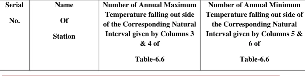
Table – 6.5
(Number of Annual Maximum Temperature and Annual Minimum Temperature falling out side of the Corresponding Natural Intervals)
Serial No.
Name Of Station
Number of Annual Maximum Temperature falling out side of the Corresponding Natural
[image:11.595.66.570.286.537.2]Interval given by Columns 3 & 4 of
Table-6.6
Number of Annual Minimum Temperature falling out side of
the Corresponding Natural Interval given by Columns 5 &
[image:11.595.67.566.629.754.2]1 DHUBRI 0 0
2 DIBRUGARH 1 0
3 GUWAHATI 0 0
4 SILCHAR 0 0
5 TEZPUR 0 0
7. DISCUSSION
The findings presented in Table – 6.2 are the 95% confidence intervals confidence intervals of the two characteristics
(1) the annual maximum temperature and
(2) the annual minimum temperature
at the 5 stations under study. This means that the annual maximum temperature and the
annual minimum temperature at each station will lie within the corresponding interval, shown
in Table – 6.2, in more than 95 years out of 100 years.
Similarly, the findings presented in Table – 6.3 and in Table – 6.4 can be interpreted. It has been found in Table – 6.5 that almost all the observed values of each of the two characteristics for each of the 5 stations lie within the corresponding natural intervals
obtained in Step – 5.6. This implies that there is no any significant cause that influences upon the changes in temperature in the context of Assam over years i.e. temperature in Assam has
not been changing (since 1969) over years significantly. The changes occurred in them are
due to the chance causes only.
The current study is based on the following assumptions:
(1) The facts and figures on the maximum temperature and the minimum
temperature collected from the stations are free from mechanical errors (i.e. errors due to the
machine / tool having unknown defect / defects and due to wrong handling of machine / tool).
(2) The facts and figures observed have been recorded correctly.
(3) Data on the characteristics mentioned in (1) are free from inconsistency.
(4) Chance errors associated to the observations in each of the characteristics are
independently and identically distributed with normal probability distribution having zero
reasonable / meaningful if these assumptions hold good. If any or all of the assumptions is
(are) not true, the findings obtained in the study are bound to be questionable.
The following results may be important to the meteorological and environmental
scientists and for the society also:
(1) It is possible to apply the area property of normal distribution to know whether
there exists any significant assignable cause in a region which forces the temperature in the
region to be changed and to determine forecasted interval value on various characteristics of
temperature with desired probability.
(2) There is no any significant cause that influence upon the changes in
temperature, in Assam, over years i.e. temperature in Assam has not been changing (since
1969) over years significantly. The changes in temperature, occurred since 1969, are due to
the chance causes only.
(3) The annual maximum temperature and the annual minimum temperature at
each of the station under study will lie within the corresponding interval, shown in
(i) Table – 6.2, in more than 95 years out of 100 years,
(ii) Table – 6.3, in more than 99 years out of 100 years and (iii) Table – 6.4, in more than 9973 years out of 10000 years.
8. REFERENCE
1. BryeWlodzimierz (1995): “The Normal Distribution : Characterizations with
Applications” Springer – Verlag, ISBN 0 – 387 – 97990 – 5.
2. Bernoulli J. (1713): “ArtsConjectandi”, ImpensisThurmisiorumFratrumBasileae. 3. Chakrabarty D. (2005a): “Probabilistic Forecasting of Time Series ”, Report ofPost
Doctoral Research Project (2002 – 2005), submitted to the University Grants Commission, New Delhi.
4. Chakrabarty D. (2005b): “ Probability: Link between the Classical Definition and the
Empirical Definition “, J. Ass. Sc. Soc., 45,June, 13-18.
5. Chakrabarty D. (2008) : “ Bernoulli’s Definition of Probability : Special Case of its
Chakrabarty's Definition ”, Int. J. Agricult. Stat. Sci., 4(1), 23 – 27.
6. De Moivre Abraham (1711): “De MensuraSortis (Latin Version)”,
PhilosophicalTransaction of the Royal Society.
8. Federer W. T. (1955): “Experimental Design”, Oxford &IBH Publication
9. Fisher R. A. and Yates F. (1938): “The Normal Probability Integral
(VIIIA)”,Statistical Tables for Biological, Agricultural and Medical Research, Sixth Edition (1982), Longman Group Limited, England, Page - 17.
10. Grant E. L. (1972): “Statistical Quality Control ”, McGraw Hill.
11. HazewinkelMichiel ed. (2001) : “ Normal Distribution ”, Encyclopedia ofMathematics, Springer, ISBN 978 – 1 – 55608 – 010 - 4.
12. Kendall M. G. and Stuart A. (1977): “Advanced Theory of Statistics ”, Vol. 1 & 2,
4thEdition, New York, Hafner Press.
13. Marsagilia George (2004) : “Evaluating the Normal Distribution”, Journal of Statistical Software, 11 (4), . http : / / www.jstatsoft.org / v11 / i05 / paper.
14. Shewhart W. A. (1931): “Economic Control of Quality of Manufactured Product ”,
Van Nastrand.
15. Stigler Stephen M. (1982) : “A Modest Proposal : A New Standard for the Normal”, The American Statistician, 36 (2), 137 – 138.
16. Walker Helen M. and Lev J. (1965): “Statistical Inference”, Oxford & IBH Publishing
Company.
17. Walker Helen M. (1985): “De Moivre on the Law of Normal Probability”, In Smith,