LINEARIZATION COEFFICIENTS FOR SHEFFER
POLYNOMIAL SETS VIA LOWERING OPERATORS
Y. BEN CHEIKH AND H. CHAGGARAReceived 16 May 2005; Revised 2 March 2006; Accepted 12 March 2006
The lowering operatorσassociated with a polynomial set{Pn}n≥0is an operator not de-pending onnand satisfying the relationσPn=nPn−1. In this paper, we express explicitly
the linearization coefficients for polynomial sets of Sheffer type using the corresponding lowering operators. We obtain some well-known results as particular cases.
Copyright © 2006 Hindawi Publishing Corporation. All rights reserved.
1. Introduction
Let ᏼbe the linear space of polynomials with complex coefficients. A polynomial se-quence{Pn}n≥0inᏼis called a polynomial set if and only if degPn=nfor all nonnegative integersn. Given two polynomial sets{Sn}n≥0and{Pn}n≥0, the so-called connection
prob-lem between them asks to find the coefficientsCm(n) in the expression:
Sn(x)= n
m=0
Cm(n)Pm(x), (1.1)
which forSn(x)=xnis known as the inversion problem for the polynomial set{Pn}n≥0.
WhenSi+j(x)=Qi(x)Rj(x) in (1.1),{Qn}nand{Rn}nbeing two polynomial sets, we are faced to the general linearization problem
Qi(x)Rj(x)= i+j
k=0
Li j(k)Pk(x). (1.2)
Particular case of this problem is the standard linearization or Clebsch-Gordan-type prob-lem
Pi(x)Pj(x)= i+j
k=0
Li j(k)Pk(x). (1.3)
The computation of the connection and linearization coefficients plays an important role
Hindawi Publishing Corporation
International Journal of Mathematics and Mathematical Sciences Volume 2006, Article ID 54263, Pages1–15
in many situations of pure and applied mathematics and also in physical and quantum chemical applications [32,33]. In particular, the study of positivity conditions ofLi j(k) has received special attention. This property has many important consequences. It gives rise to a convolution structure associated with the polynomial set{Pn}n≥0[8,9,19,36]. Several sufficient conditions for the sign properties to hold have been derived in [6,7,37, 38]. The literature on this topic is extremely vast and a wide variety of methods, based on specific properties of the involved polynomials, have been devised for computing the linearization coefficientsLi j(k) either in closed form or by means of recursive relations (usually ink) [10,26,27], exploiting for this purpose several of their specific properties: recurrence relation [24], generating function [3,7, 15,16,22], orthogonality weights and Rodrigue’s formula [1,5], inversion formulas [4,29], and so forth. A combinatorial approach to solve the linearization problems was also given in [21,28,39].
A general method, based on lowering operators, was developed by the authors [13,14] to solve connection problems. The purpose of this work is to show that such a technique can likewise be used to treat linearization problems.
The outline of the paper is as follows. InSection 2, we give a result for a general lin-earization problem. Then we prove a useful lemma, generalizing the Leibniz formula, to express explicitly the standard linearization coefficients for Sheffer polynomial sets (Theorem 2.6). InSection 3, for practical uses of the main result, we give the standard linearization coefficients for some well-known basic Sheffer polynomial sets. Finally, in Section 4, we applyTheorem 2.6to orthogonal Sheffer polynomial sets.
2. Linearization coefficients
2.1. A general result. Denote byΛ(−1)the space of operatorsσ acting on analytic func-tions that reduce the degree of every polynomial by exactly one andσ(1)=0.
It was shown, by the first author, that every polynomial set is quasi-monomial [12]. That is to say, there exist a lowering operatorσ and a raising operatorτ, independent of n, such that
σPn=nPn−1, τPn=Pn+1, n=1, 2,. . . . (2.1)
Definition 2.1. Letσ∈Λ(−1)and let{Pn}n
≥0be a polynomial set.{Pn}n≥0is called a σ-Appell polynomial set if and only if
σPn
=nPn−1, n=1, 2,. . . . (2.2)
Definition 2.2. Letσ ∈Λ(−1). A polynomial set {Bn}n
≥0 is called the sequence of basic polynomials forσif and only if
(i){Bn}n≥0is aσ-Appell polynomial set; (ii)Bn(0)=δ0,n,n=0, 1,. . . .
Theorem 2.3 [11]. Let{Pn}n≥0 be a polynomial set. Then there exist a uniqueσ∈Λ(−1) and a unique power seriesA(t)=∞k=0antn,a0=0, such that{Pn}n≥0is aσ-Appell poly-nomial set and
A(σ)Bn
=Pn, n=0, 1,. . ., (2.3)
where{Bn}n≥0is the sequence of basic polynomials forσ.
Call{Pn}n≥0aσ-Appell polynomial set of transfer power seriesA. Aσ-Appell polynomial set of transfer power seriesAis generated by
G(x,t)=A(t)G0(x,t)=
∞
n=0 Pn(x)
n! t
n, (2.4)
whereG0(x,t) is a solution of the system
σG0(x,t)=tG0(x,t), G0(x, 0)=1, (2.5)
and conversely.
Letᏼ be the algebraic dual ofᏼ. We denote byᏸ,f the effect of the functional
ᏸ∈ᏼ on the polynomial f ∈ᏼ. Let{Pn}n
≥0 be a polynomial set. Its dual sequence {Pn}n≥0is defined by
Pn,Pm
=δn,m, n,m≥0. (2.6)
When{Pn}n≥0is aσ-Appell polynomial set of transfer power seriesA, an explicit expres-sion of its dual sequence was given in [11] by
Pn,f= 1 n!σ
nA(σ )(f)(x) x=0,
n=0, 1,. . ., f ∈ᏼ, (2.7)
whereA(t) =1/A(t).
Combining (1.2), (2.6), and (2.7), we state the following general result. Theorem 2.4. Letσ∈Λ(−1) and{Pn}n
≥0be aσ-Appell polynomial set of transfer power seriesA. Then the general linearization coefficients in (1.2) are given by
Li j(k)= 1 k!σ
kA(σ )Q iRj
(0), i,j=0, 1,. . .,k=0, 1,. . .,i+j. (2.8)
Next, in this paper, we limit ourselves to standard case for Sheffer polynomial sets case.
2.2. Sheffer polynomials. Recall that a polynomial set{Pn}n≥0 is said to be of Sheffer typeA-zero (Sheffer polynomial set, for shorter,) if and only if it has a generating function of the form [25,30]
A(t) exp(xC(t))=
∞
n=0 Pn(x)
n! t
whereAandCare two formal power series:
A(t)=
∞
k=0
aktk, a0=0, C(t)=
∞
k=0
cktk+1, c0=0. (2.10)
It was shown in [12] that a Sheffer polynomial set generated by (2.9) isσ-Appell polyno-mial set of transfer power seriesA, whereσ=C∗(D), D=d/dx, andC∗is the inverse of C; that is,C∗(C(t))=C(C∗(t))=t.
IfC(t)=t, we haveσ=D. That corresponds to Appell polynomial sets [2]. In order to apply (2.8) to Sheffer polynomial sets we need the following. Lemma 2.5 (generalized Leibniz formula). Letσ∈Λ(−1)and let{Bn}n
≥0be the sequence of basic polynomials forσ. Suppose thatσcommutates with the derivative operator D. Let f andgbe two formal power series. Then,
σnf(z)g(z)=
∞
m=n m
k=0
ck,m(n)σkf(z)σm−kg(z), (2.11)
where
ck,m(n)= 1 k!(m−k)!σ
n(B kBm−k)
x=0
. (2.12)
Proof. Letz0∈C. Let us define the translation operatorsTz0 byTz0f(z)=ez0Df(z)= f(z+z0). Sinceσcommutates withTz0, f andghave the formal power expansions:
f(z)=Tz0f(z−z0)= ∞
m=0
σmf(z0)
m! Bm(z−z0), g(z)=
∞
m=0
σmg(z0)
m! Bm(z−z0), (2.13)
by virtue of (2.7). So
σnf(z)g(z)= ∞ m=n
m
k=0
σkf(z0) k!
σm−kg(z0) (m−k)! σ
nB
k(z−z0)Bm−k(z−z0)
, (2.14)
sinceσn(B
k(z−z0)Bm−k(z−z0))=0 ifm < n. Putz=z0in (2.14), we deduce (2.11) since
z0is arbitrary.
For the particular caseσ=D, the corresponding basic sequence isBn(x)=xn. Then the coefficients in (2.12) are given by
ck,m(n)=k!(m1−k)!Dn(xm)
x=0= n!
k!(m−k)!δn,m, (2.15) and (2.11) is reduced to the well-known Leibniz formula
Dnf(z)g(z)= n
k=0
n k
As every Sheffer polynomial set generated by (2.9) may be viewed as aσ-Appell polyno-mial set of transfer power seriesAwhereσ=C∗(D), we use this property to state our following main result.
Theorem 2.6. The linearization coefficients in (1.3) with{Pn}n≥0a Sheffer polynomial set generated by (2.9) are given by
Li j(k)=
m≥k m
p=0
i p
j m−p
lp,m−p(k)A
C∗(D)Pi−pPj−m+p(x) x=0
, (2.17)
wherelnm(k) are the standard linearization coefficients for the corresponding basic sequence generated by
1 k!C∗
kC(t) +C(s)= n,m
lnm(k) n!m! t
nsm. (2.18)
Proof. {Pn}n≥0is aσ-Appell polynomial set of transfer power seriesA, whereσ=C∗(D). Then by virtue ofTheorem 2.4and (2.11) we derive (2.17).
The basic sequence{Bn}n≥0is aσ-Appell polynomial set of transfer power series 1. So according to (2.8) and (2.16), we have
li j(k)=k!1σk(BiBj)
x=0= 1 k!C
∗k(D)(B iBj)
x=0 =1
k!
n≥k
αn,kDk(BiBj)
x=0
, whereC∗k(t)= n≥k
αn,ktn,
=1 k!
n≥k αn,k
n
p=0
n p
DpBiDk−pBj x=0
=k!1 n≥k
αn,k n
p=0
n p
C(σ)pBiC(σ)k−pBj x=0
=1 k!
n≥k αn,k
C(σ)(Bi) +C(σ)(Bj) n
x=0
=1 k!C
∗kC(σ(B i)
+C(σ(Bj) x=0
.
(2.19)
Put (1/k!)C∗k(C(t) +C(s))=
n,man,m(k)tnsm. It follows from (2.19) andDefinition 2.2 that
li,j(k)=1 k!
n,m
an,m(k)σn(Bi)σm(Bj)
x=0 =1
k!
n,m
an,m(k)(i−i!n)!Bi−n(0) j!
(j−m)!Bj−m(0)
x=0=
i!j!ai,j(k),
(2.20)
Remark 2.7. A similar proof may be used to express general linearization coefficients in (1.2) where the involved three polynomial sets are of Sheffer type.
Next, inSection 3, we use (2.18) to express explicitly the standard linearization coeffi -cients for some well-known basic Sheffer polynomial sets. Then, inSection 4, in order to show the efficiency of the proposed approach, we applyTheorem 2.6to orthogonal Shef-fer polynomial sets to derive some already obtained results in the literature by alternative methods.
3. Linearization coefficients for basic polynomials
3.1. Stirling polynomials. The Stirling polynomial set{x[n]=x(x−1)···(x−n+ 1)}n
≥0 is generated by
(1 +t)x=
∞
n=0 x[n]
n! t
n. (3.1)
For this case we haveC(t)=Log(1 +t) andC∗(t)=et−1. It follows that{x[n]}n
≥0is aΔ-Appell polynomial set, whereΔ=eD−1 is the difference operator, and
1 k!C
∗kC(t) +C(s)=1
k!(t+s+st) k=
n,m
tm+k−nsk−m (k−n)!(n−m)!m!
=
i,j
tisj
(k−j)!(k−i)!(i+j−k)!.
(3.2)
Then
x[i]x[j]= min(i,j)
k=0 k!
i k
j k
x[i+j−k]. (3.3)
According to (3.3), the following relations can be derived
x n
x m
=
min(n,m)
k=0
(n+m−k)! (n−k)!(m−k)!k!
x n+m−k
,
(x)n(x)m= min(n,m)
k=0
(−1)kk!
n k
m
k
(x)n+m−k,
(3.4)
where (x)n=x(x+ 1)···(x+n−1).
Also, from (3.3), one can see that (2.11) contains as a particular case the well-known Jordan formula [20]
Δn(f g)(z)= n
k=0
n k
In fact, for the special caseσ=Δ, the corresponding basic sequence isBn(x)=x[n]. Then (2.12) is reduced to
ck,m(n)= n!
k!(m−k)!lk,m−k(n)=
n!
(n−k)!(n−m)!(m+k−n)!. (3.6) It follows from (2.11) and (3.6) that
Δnf(z)g(z)=∞ m=0
m
k=0
ck,mΔkf(z)Δm−kg(z)=
∞
k=0 n! k!Δ
kf(z) ∞
m=0 lk,m(n)
m! Δ
mg(z)
=
∞
k=0 Δkf(z)
∞
m=0
n!
(n−k)!(n−m)!(m+k−n)!Δ mg(z)
=
∞
k=0
n k
Δkf(z)Δn−k ∞
p=0
k p
Δpg(z)
,
(3.7)
which, in view of the expansion formula [20]
g(z+a)=
∞
p=0
a p
Δpg(z), (3.8)
gives (3.5).
3.2. Basic Laguerre polynomials. The basic Laguerre polynomials{Ln(x)}n≥0 are gen-erated by
ex(t/(t−1))=∞ n=0
Ln(x)tn. (3.9)
ThenC(t)=C∗(t)=t/(t−1).It follows that{n!Ln(x)}n≥0is aσ-Appell polynomial set, whereσ=D/(D−1) is the Laguerre operator.
For this case we have 1
k!C
∗kC(t) +C(s)=1 k!
t+s−2st 1−st
k
=
i,j
n≥0
(k)n(−2)i+j−k−2n
(n+k−j)!(n+k−i)!(i+j−k−2n)!t isj.
(3.10)
Then
li j(k)=
n≥0
(k)nk!(−2)i+j−k−2n
n!(n+k−i)!(n+k−j)!(i+j−k−2n)!
= (−2)i+j−kk!
(i+j−k)!(k−i)!(k−j)!3F2 ⎛ ⎜ ⎝k,
k−i−j
2 ,
k−i−j+ 1 2 k−i+ 1,k−j+ 1
; 1 ⎞ ⎟ ⎠.
3.3. Basic Meixner polynomials. The basic Meixner polynomial set{Pn(x)}n≥0is gener-ated by
exln((1−t/a)/(1−t))=∞ n=0
Pn(x) n! t
n. (3.12)
For this case we have
C(t)=ln
1−t/a 1−t
, C∗(t)= et−1
et−1/a. (3.13)
It follows that{Pn(x)}n≥0is aσ-Appell polynomial set, whereσ=(eD−1)/(eD−1/a), and
1 k!C
∗kC(t) +C(s)=1 k!
t
+s−(1 + 1/a)st 1−st/a
k
=
i,j
n≥0
(k)n(−1−1/a)i+j+k−2n
n!an(n+k−j)!(n+k−i)!(i+j−k−2n)!tisj.
(3.14)
Then
li j(k)=
n≥0
(k)ni!j!(−1−1/a)i+j−k−2n n!an(n+k−i)!(n+k−j)!(i+j−k−2n)!
= i!j!(−1−1/a)i+j−k (i+j−k)!(k−i)!(k−j)!3F2
⎛ ⎜ ⎝k,
k−i−j
2 ,
k−i−j+ 1 2 k−i+ 1,k−j+ 1
; 4a (a+ 1)2
⎞ ⎟ ⎠.
(3.15)
3.4. Basic Meixner-Pollaczek polynomials. The basic Meixner-Pollaczek polynomial set
{Pn(x)}n≥0is generated by
exarctan(t/(1+δt))=
∞
n=0 Pn(x)
n! t
n. (3.16)
For this case we have
C(t)=arctan t
1 +δt, C
∗(t)= tant
1−δtant. (3.17)
It follows that{Pn(x)}n≥0is aσ-Appell polynomial set, whereσ=tanD/(1−δtanD) and
1 k!C
∗kC(t) +C(s)=1 k!
t+s+ 2δst 1−(1 +δ2)st
k
=
i,j
n≥0
(k)n(1 +δ2)n(2δ)i+j−k−2n
n!(n+k−j)!(n+k−i)!(i+j−k−2n)!t isj.
Then
li j(k)=
n≥0
(k)n(1 +δ2)ni!j!(2δ)i+j−k−2n n!(n+k−i)!(n+k−j)!(i+j−k−2n)!
= i!j!(2δ)i+j−k
(i+j−k)!(k−i)!(k−j)!3F2 ⎛ ⎜ ⎝k,
k−i−j
2 ,
k−i−j+ 1 2 k−i+ 1,k−j+ 1
;1 +δ 2
δ2 ⎞ ⎟ ⎠.
(3.19)
4. Orthogonal Sheffer polynomials
Let{Pn}n≥0 be an orthogonalσ-Appell polynomial set of transfer power seriesA. The linear functionalᏸfor which the orthogonality holds is given by [34]
ᏸ,f =A(σ)( f)(0). (4.1)
We use this relation andTheorem 2.6to state the following.
Corollary 4.1. The linearization coefficients in (1.3) for{Pn}n≥0an orthogonalσ-Appell polynomial set of transfer power seriesAof Sheffer type are given by
Li j(k)=
2s≤i+j−k
i s
j s
li−s,j−s(k)Is, (4.2)
whereIs= ᏸ,PsPs =A(σ)(P s2)(x)|x=0 andli j are the standard linearization coefficients for the corresponding basic sequence.
An immediate consequence of this result is the following.
Corollary 4.2. A sufficient condition to ensure the positivity of the standard linearization coefficients for an orthogonal Sheffer polynomial set is the positivity of those associated with the corresponding basic sequence.
It follows, from the results obtained inSection 3, that the standard linearization co-efficients for Hermite, Charlier, monic Laguerre polynomials {(−1)nn!Lα
n(x)}n≥0, and
Meixner-Pollaczek polynomials are positive.
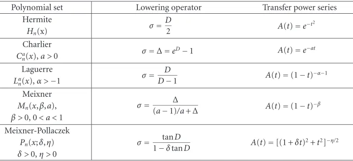
Let us return now to Corollary 4.1to mention that this result concerns exactly five classes of Sheffer polynomials according to Meixner characterization [17]. InTable 4.1, we recall these classes with the corresponding lowering operators and transfer power se-ries according to our analysis.
Next, for each case, we use (4.2) to express explicitly the corresponding standard lin-earization coefficients in terms of hypergeometric series.
4.1. Hermite polynomials. The Hermite polynomials{Hn}n≥0are generated by
e−t2e2xt=
∞
n=0 Hn(x)
n! t
Table 4.1. Orthogonal Sheffer polynomial sets.
Polynomial set Lowering operator Transfer power series Hermite
σ=D
2 A(t)=e
−t2
Hn(x)
Charlier
σ=Δ=eD−1 A(t)=e−at
Ca
n(x),a >0
Laguerre
σ= D
D−1 A(t)=(1−t) −α−1 Lα
n(x),α >−1
Meixner
σ= Δ
(a−1)/a+Δ A(t)=(1−t)−β Mn(x,β,a),
β >0, 0< a <1 Meixner-Pollaczek
σ= tanD
1−δtanD A(t)=[(1 +δt) 2+t2]−η/2 Pn(x;δ,η)
δ >0,η >0
Thenσ=D/2 andA(t)=e−t2
. Since the corresponding basic sequence is{(2x)n}n
≥0, we
getli j(k)=δi+j,k. The linear functional for which the orthogonality holds is [34]
A(σ)(f)(0)=exp(σ2)(f)(0)=√1 π
+∞
−∞e −x2
f(x)dx. (4.4)
Then we have [17]Is=s!2s. According to (4.2), we deduce [18]
Li j(k)= ⎧ ⎪ ⎪ ⎨ ⎪ ⎪ ⎩
i s
j s
2ss! if k=i+j−2s,
0 otherwise.
(4.5)
4.2. Charlier polynomials. The Charlier polynomials{Ca
n}n≥0are generated by
e−at(1 +t)x=
∞
n=0 Ca
n(x) n! t
n. (4.6)
Thenσ=ΔandA(t)=e−at. Since the corresponding basic sequence is the Stirling poly-nomial set{x[n]}n
≥0, we haveli j(k)=k! i
i+j−k
j
i+j−k
by virtue of (3.3). The linear func-tional for which the orthogonality holds is [34]
A(σ)(f)(0)=exp(aΔ)(f)(0)=e−a
∞
j=0 aj
Then we have [17]Is=ass!. According to (4.2), we obtain [39]
Li j(k)=
s≥0
i!j!as
(s+k−i)!(s+k−j)!(s)!(i+j−k−2s)!
= i!j!
(i+j−k)!(k−i)!(k−j)!2F2 ⎛ ⎜ ⎝
k−i−j
2 ,
k−i−j+ 1 2 k−i+ 1,k−j+ 1
; 4a ⎞ ⎟ ⎠.
(4.8)
4.3. Laguerre polynomials. The Laguerre polynomials{Lαn}n
≥0are generated by [17]
(1−t)−α−1exp
x t t−1
=
∞
n=0
Lαn(x)tn. (4.9)
Then the lowering and transfer operators for{n!Lα
n}n≥0 are, respectively,σ=D/(D−1) andA(σ)=(1−σ)−α−1. The linear functional for which the orthogonality holds is [34]
A(σ)(f)(0)=1−σα+1(f)(0)=Γ(α1 + 1)
+∞
0 f(x)x
αe−xdx, α >−1. (4.10)
For this case we have [17,23]Is=s!(α+ 1)s.
According to (3.11) and (4.2), we deduce the linearization coefficients for{Lα n}n≥0,
Li j(k)=
−2i+j−k k!
n,s
2−2(n+s)k n
α+ 1s
n!s!(n+s) +k−i!(n+s) +k−j)!(i+j−k−2(n+s)!, (4.11)
which, in view of the well-known relationship [31,35]:
n,m
(ρ)n(σ)mcn+m
m!n! x
n+m= n
(ρ+σ)ncn
n! x
n, {cn}being a sequence of complex numbers, (4.12)
assumes the form [28]
Li j(k)=(−2) i+j−k k!
p≥0
(α+ 1 +k)p2−2p
p!(p+k−i)!(p+k−j)!(i+j−k−2p)!
= (−2)i+j−k
k!(i+j−k)!(k−i)!(k−j)!3F2 ⎛ ⎜
⎝k+α+ 1,
k−i−j
2 ,
k−i−j+ 1 2 k−i+ 1,k−j+ 1
; 1 ⎞ ⎟ ⎠.
(4.13)
4.4. Meixner polynomials. The Meixner polynomial set{Mn(x;β,a)}n≥0is generated by [17]
(1−t)−β
1−t/a 1−t
x =
∞
n=0
Mn(x;β,a)t n
It follows thatσ=(eD−1)/(eD−1/a) and A(t)=(1−t)−β. The linear functional for which the orthogonality holds is [34]
A(σ)(f)(0)=1−σβ(f)(0)=1−aβ
∞
j=0 (β)j
j! a
jf(j). (4.15)
For this case we have [18]Is=s!(β)sa−s. According to (3.15), (4.2), and (4.12) we obtain [9]
Li j(k)=i!j!
−1−1 a
i+j−k
p≥0
β+kp1 +a−2pap
p!(p+k−i)!(p+k−j)!(i+j−k−2p)!
= i!j!
−1−1/a i+j−k
(i+j−k)!(k−i)!(k−j)!3F2 ⎛ ⎜ ⎝k+β,
k−i−j
2 ,
k−i−j+ 1 2 k−i+ 1,k−j+ 1
; 4a (a+ 1)2
⎞ ⎟ ⎠.
(4.16)
So, the linearization coefficients alternate in sign just as in the Laguerre polynomial set case.
4.5. Meixner-Pollaczek polynomials. The Meixner-Pollaczek polynomials are generated
by [17]
1 +δt2+t2−η/2exarctan(t/(1+δt))=
∞
n=0
Pn(x,δ,η)
n! t
n. (4.17)
Then we have
σ= tanD
1−δtanD, A(t)=
1 +δt2+t2−η/2. (4.18)
To obtain the effect of the linear functionalA(σ) on analytic functions, we need the fol- lowing relation [39]:
1 πΓ(ρ)
+∞
−∞e
−(π−2t)x Γρ+ix 2
2dx=2 sint−ρ, ρ >0. (4.19)
It follows from (4.18) that
Aσ(f)=(cosD−δsinD)−η(f)=
sinπ/2 +D+ arctanδ sinπ/2 + arctanδ
−η (f)
= +∞
−∞ f(x)ω(x)dx
+∞ −∞ω(x)dx
,
where ω(x)=[Γ(η/2)]−2|Γ(η+ix/2)|2exp (−xtan−1δ). So we have [17, 23] I
s=(δ2+ 1)ss!(η)
s. According to (3.19), (4.2), and (4.12), we obtain [39]
Li j(k)=i!j!(2δ)i+j−k
p≥0
η+kp2δ−2p1 +δ2p p!(p+k−i)!(p+k−j)!(i+j−k−2p)!
= i!j!
2δi+j−k
(i+j−k)!(k−i)!(k−j)!3F2 ⎛ ⎜ ⎝k+η,
k−i−j
2 ,
k−i−j+ 1 2 k−i+ 1,k−j+ 1
;1 +δ 2
δ2 ⎞ ⎟ ⎠.
(4.21)
Takingδ→0 andη=2λin (4.21) and using the well-known relation [35], namely, −2k+ 1
2
k=
−1k(2k)!
22kk!, k=0, 1, 2,. . ., (4.22) we obtain [3]
p(iλ)(x)p(jλ)(x)= min(i,j)
k=0
Γ(i+j−2k+ 2λ+ 1)(i+j−2k)! k!(i−k)!(j−k)! p
(λ)
i+j−2k(x), (4.23)
where p(nλ)(x)=(1/n!)Pn(x; 0, 2λ) designates the symmetric Meixner-Pollaczek polyno-mials.
References
[1] R. ´Alvarez-Nodarse, R. J. Y´a˜nez, and J. S. Dehesa, Modified Clebsch-Gordan-type expansions for products of discrete hypergeometric polynomials, Journal of Computational and Applied Mathe-matics 89 (1998), no. 1, 171–197.
[2] P. Appell, Sur une classe de polynˆomes, Annales Scientifiques de l’ ´Ecole Normale Sup´erieure 9 (1880), no. 2, 119–144.
[3] T. K. Araaya, Linearization and connection problems for the symmetric Meixner-Pollaczek polyno-mials, Uppsala University (2003), 59–70.
[4] I. Area, E. Godoy, A. Ronveaux, and A. Zarzo, Solving connection and linearization problems within the Askey scheme and itsq-analogue via inversion formulas, Journal of Computational and Applied Mathematics 133 (2001), no. 1-2, 151–162.
[5] P. L. Art´es, J. S. Dehesa, A. Mart´ınez-Finkelshtein, and J. S´anchez-Ruiz, Linearization and con-nection coefficients for hypergeometric-type polynomials, Journal of Computational and Applied Mathematics 99 (1998), no. 1-2, 15–26.
[6] R. Askey, Orthogonal polynomials and positivity, Studies in Applied Mathematics, Special Func-tions and Wave Propagation, vol. 6, SIAM, Pennsylvania, 1970, pp. 64–85.
[7] , Orthogonal Polynomials and Special Functions, CBMS Regional Conference Series, vol. 21, SIAM, Pennsylvania, 1975.
[8] R. Askey and G. Gasper, Linearization of the product of Jacobi polynomials. III, Canadian Journal of Mathematics 23 (1971), 332–338.
[9] , Convolution structures for Laguerre polynomials, Journal d’Analyse Math´ematique 31 (1977), 48–68.
[11] Y. Ben Cheikh, On obtaining dual sequences via quasi-monomiality, Georgian Mathematical Jour-nal 9 (2002), no. 3, 413–422.
[12] , Some results on quasi-monomiality, Applied Mathematics and Computation 141 (2003), no. 1, 63–76.
[13] Y. Ben Cheikh and H. Chaggara, Connection problems via lowering operators, Journal of Compu-tational and Applied Mathematics 178 (2005), no. 1-2, 45–61.
[14] , Connection coefficients between Boas-Buck polynomial sets, Journal of Mathematical Analysis and Applications 319 (2006), no. 2, 665–689.
[15] L. Carlitz, The product of certain polynomials analogous to the Hermite polynomials, The American Mathematical Monthly 64 (1957), 723–725.
[16] , Products of Appell polynomials, Collectanea Mathematica 15 (1963), 245–258. [17] T. S. Chihara, An Introduction to Orthogonal Polynomials, Gordon and Breach, New York, 1978. [18] A. Erd´elyi, W. Magnus, F. Oberhettinger, and F. G. Tricomi, Higher Transcendental Functions.
Vols. I, II, McGraw-Hill, New York, 1953.
[19] G. Gasper, Linearization of the product of Jacobi polynomials. I, Canadian Journal of Mathematics 22 (1970), 171–175.
[20] C. Jordan, Calculus of Finite Differences, 2nd ed., Chelsea, New York, 1960.
[21] D. Kim and J. Zeng, A combinatorial formula for the linearization coefficients of general Sheffer polynomials, European Journal of Combinatorics 22 (2001), no. 3, 313–332.
[22] H. Kleindienst and A. L¨uchow, Multiplication theorems for orthogonal polynomials, International Journal of Quantum Chemistry 48 (1993), no. 4, 239–247.
[23] R. Koekoek and R. F. Swarrtow, The Askey-scheme of hypergeometric orthogonal polynomials and itsq-analogue, Tech. Rep. 98–17, Faculty of the Technical Mathematics and Informatics, Delft University of Technology, Delft, 1998.
[24] C. Markett, Linearization of the product of symmetric orthogonal polynomials, Constructive Ap-proximation 10 (1994), no. 3, 317–338.
[25] E. D. Rainville, Special Functions, Macmillan, New York, 1960.
[26] A. Ronveaux, Orthogonal polynomials: connection and linearization coefficients, Proceedings of the International Workshop on Orthogonal Polynomials in Mathematical Physics (M. Alfano, R. ´Alvarez-Nodarse, G. L ´opez Lagomasino, and F. Marcell´an, eds.), Madrid, June 1996. [27] A. Ronveaux, M. N. Hounkonnou, and S. Belmehdi, Generalized linearization problems, Journal
of Physics. A: Mathematical and General 28 (1995), no. 15, 4423–4430.
[28] J. S´anchez-Ruiz, P. L. Art´es, A. Mart´ınez-Finkelshtein, and J. S. Dehesa, Linearization problems of hypergeometric polynomials in quantum physics, Proceedings of the Melfi Workshop on Advanced Special Functions and Applications (G. Dattoli, H. M. Srivastava, and D. Cocolicchio, eds.), Rome, May 1999.
[29] J. S´anchez-Ruiz and J. S. Dehesa, Some connection and linearization problems for polynomials in and beyond the Askey scheme, Journal of Computational and Applied Mathematics 133 (2001), no. 1-2, 579–591.
[30] I. M. Sheffer, Some properties of polynomial sets of type zero, Duke Mathematical Journal 5 (1939), no. 3, 590–622.
[31] H. M. Srivastava, On the reducibility of Appell’s functionF4, Canadian Mathematical Bulletin 16 (1973), 295–298.
[32] , A unified theory of polynomial expansions and their applications involving Clebsch-Gordan type linearization relations and Neumann series, Astrophysics and Space Science 150 (1988), no. 2, 251–266.
[34] H. M. Srivastava and Y. Ben Cheikh, Orthogonality of some polynomial sets via quasi-monomial-ity, Applied Mathematics and Computation 141 (2003), no. 2-3, 415–425.
[35] H. M. Srivastava and H. L. Manocha, A Treatise on Generating Functions, John Willey & Sons, New York; Brisbane, Toronto, 1984.
[36] R. Szwarc, Convolution structures associated with orthogonal polynomials, Journal of Mathemati-cal Analysis and Applications 170 (1992), no. 1, 158–170.
[37] , Nonnegative linearization and quadratic transformation of Askey-Wilson polynomials, Canadian Mathematical Bulletin 39 (1996), no. 2, 241–249.
[38] , A necessary and sufficient condition for nonnegative product linearization of orthogonal polynomials, Constructive Approximation 19 (2003), no. 4, 565–573.
[39] J. Zeng, Weighted derangements and the linearization coefficients of orthogonal Sheffer polynomials, Proceedings of the London Mathematical Society. Third Series 65 (1992), no. 1, 1–22.
Y. Ben Cheikh: D´epartement de Math´ematiques, Facult´e des Sciences de Monastir, Universit´e de Monastir, 5019 Monastir, Tunisia
E-mail address:[email protected]
H. Chaggara: D´epartement de Pr´eparation en Math-Physique, Institut Pr´eparatoire aux ´Etudes d’Ing´enieur de Monastir, 5019 Monastir, Tunisia