Nonreflecting boundary conditions obtained from equivalent sources for time dependent scattering problems

(1)

Nonreflecting Boundary Conditions Obtained From

Equivalent Sources For Time-Dependent

Scattering Problems

Thesis by

David Hoch

In Partial Fulfillment of the Requirements

for the Degree of

Doctor of Philosophy

California Institute of Technology

Pasadena, California

2008

(2)

(3)

(4)

Acknowledgments

I would like to thank my advisor, Professor Oscar P. Bruno, for sharing his vast experience, providing careful guidance and unwavering support, and for his continual encouragement. He introduced me to many advanced spectral methods and suggested the topic of this thesis. I enjoyed the many discussions we had, both mathematical and nonmathematical, which I will always keep in good memory.

I wish to express my gratitude to Professor Tom Y. Hou for encouraging me to join the Applied and Computational Mathematics Program at Caltech and for his kind support especially during the first graduate year.

Special thanks are due to Professor Christophe Geuzaine, for providing me with Gmsh, a three-dimensional finite element mesh generator he and his coworkers developed, which can be downloaded from http://geuz.org/gmsh. He also helped me to integrate the mesh generator into my existing code and provided very useful C++ classes.

Tim Elling confirmed and provided certain numerical results in connection with equivalent sources in Appendix B.2 which I am very thankful for.

I would also like to extend my thanks to Professor Thomas Hagstrom for helpful suggestions and references to related recent works.

Our talented and generous systems manager Chad Schmutzer was always willing and ready to solve the countless unpredictable problems I encountered with computers, and I owe him a special thank you for all the time he saved me.

For her thoughtfulness, kindness, and friendliness, I would like to thank our department’s adminis-trator, Ms. Sheila Shull. I also wish to thank the other faculty and staff of Caltech with whom I have had the privilege of interacting and especially the rest of my thesis committee, Professors Dan Meiron and Joe Shepherd.

(5)

v

my decision to pursue a scientific career in the United States. Dr. Schwab taught me the basics of partial differential equations and hp finite elements. Dr. Grote introduced me to the world of nonreflecting boundary conditions.

(6)

Abstract

In many engineering applications, scattering of acoustic or electromagnetic waves from a body of arbi-trary shape is considered in an infinite medium. Solving the underlying partial differential equations with a standard numerical method such as finite elements or finite differences requires truncating the unbounded domain of definition into a finite computational region. As a consequence, an appropriate boundary condition must be prescribed at the artificial boundary. Many approaches have been proposed for this fundamental problem in the field of wave scattering. All of them fall into one of three main categories.

The first class of methods is based on mathematical approximations or physical heuristics. These boundary conditions are often local in space and time, therefore easy to implement and run in short computing times. However, these approaches give rise to spurious reflections at the artificial boundary, no matter how refined the discretization is, which travel back into the computational domain and corrupt the solution.

A second group consists of accurate and convergent methods. However, these formulations are usually nonlocal in time and space, thus harder to implement and often more expensive than the computation of the interior scheme itself.

Finally, there are methods which are accurate and fast. These approaches are often local in time, and the nonlocality in space is confined to a closed surface rather than the whole computational domain. The drawback of these approaches lies in the fact that the outer boundary must be taken to be either a sphere, a plane, or a cylinder. For many applications of interest, this may require use of a computational domain much larger than actually needed, which leads to an expensive overall numerical scheme.

(7)

vii

(8)

List of Figures

1.1 A typical time-dependent scattering problem . . . 2

3.1 The two discretized faces in three dimensions . . . 13 3.2 The error EP(HC) as a function ofHC at P = [0,1.25,1.26]t

for different values ofH. . . 16 3.3 The error E(P) as a function ofP = [0, l,0]t

for two different values ofHC . . . 17 3.4 The mesh size ∆S as a function of the wave numberk and the panel length H to obtain

at least O₍₁₀−6) accuracy in the field values . . . 21 3.5 The number of equivalent sources S along one panel length as a function of the wave

number k and the panel lengthH to obtain at least O₍₁₀−6) accuracy in the field values . 21 3.6 Hardest case: The mesh size ∆S in relation to the wave number k and the panel length

H to obtain at least O₍₁₀−5) accuracy in the field values . . . 24 3.7 Hardest case: The number of equivalent sourcesS along one panel length in dependence

of the wave numberk and the panel lengthH to obtain at leastO₍₁₀−5) accuracy in the field values . . . 25 3.8 Hardest case: The number of equivalent sourcesS along one panel length in dependence

of the wave numberk and the panel lengthH to obtain at leastO₍₁₀−5) accuracy in the field values . . . 25 3.9 Hardest case: Plots 3.7 and 3.8 combined . . . 26 3.10 Hardest case: The number of collocation pointsC in dependence of the wave number k

(12)

3.13 Solution (top), its first (center), and second (bottom) time derivative at [0,0,0.1876]. The crosses correspond to the numerical values, the solid line is the exact solution. . . 34 3.14 Graphical development of the data at the collocation pointxC. The interior solver needs

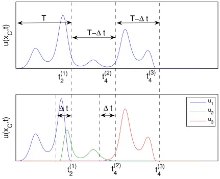
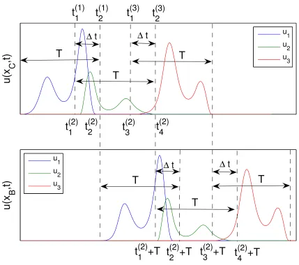
to be interrupted at the time t(1)₂ (top). The accumulated data at xC is multiplied by w₁ (bottom). The equivalent source Algorithm 3.2.1 evaluates the wave packetu₁ at xB, and the interior solver can be applied to compute the field at xC up to the time t(2)₄ (top); compare also with Figure 3.15. The wave packet u₂ is constructed atx_C (bottom), and Algorithm 3.2.1 evaluates the wave u2 at xB; using the interior solver again leads to gathered data atx_C up to the timet(3)

4 (top), which can be split intou3by an appropriate window function w3 (bottom). . . 38 3.15 Graphical development of evaluating the boundary data atxB: Given the solution from

the interior solver at x_C up to the time t(1)

2 , the wave packet u1 is constructed (top), which is evaluated at all boundary points xB with Algorithm 3.2.1 (bottom). Based on the information onB,the interior solver computes uup to timet(2)₄ =t(2)₁ +T . The POU at xC gives u₂ (top), and the arrival of this wave packet at xB can be computed with Algorithm 3.2.1 again (bottom). Note that by superposition of u₁ and u₂ at x_B, new boundary data foru are known from t(2)₁ +T to t(2)₃ +T: this enables the interior solver to evaluate u up to the time t(2)₃ +T in the whole computational domain Ω (top). This leads to an iterative process. . . 39 3.16 The continuation method is applied to the red discrete data in [0,3] to the extended

domain [0,6], resulting in the blue periodic solution. . . 44 3.17 The continuation method for different value ofN and M.Note the significant differences

of the functions in the extension domains. The blue graph corresponds to the exact solution. By construction, the approximated solution (green) matches the blue to a high accuracy in the domain [0,3] (compare with Table 3.6). . . 45 3.18 Left: Geometry of the problem. Right: Fourier continuation method applied to the

(13)

LIST OF FIGURES xiii

3.19 Top: The infinitesimal wave which travels the minimum distance rmin from SC to B. Middle: The infinitesimal wave that travels the maximum distance rmax from SC to B. Bottom: Overlapping the two extreme cases gives the validity of the domain of the field at B. . . 50

3.20 The initial data and its periodic extension at the collocation points . . . 52

3.21 The blue curve shows the exact wave function; the green curve is the numerical solution obtained by extending the data periodically with the continuation method at the colloca-tion points, obtaining the corresponding equivalent sources on the two faces D1 and D2, and evaluating the field with these sources at the shown points. . . 54

4.1 Geometry of the global problem: The computational domain Ω with inner boundary Γ and outer boundaryB. The Cartesian gridτH splits the cuboid into cubes, and the Kirchhoff surfaceS embeds the scatterer Γ and is compromised of specially selected faces ofτH. . . 57 4.2 Geometry for local panel Sj. The two two-face pairsD_(j,1)(l) ∪D(l)_(j,2), l∈ {1,2}, are

perpen-dicular toSj and are of edge sizeH. . . 58 4.3 Graphical illustration of the local problem: The continuation method is applied to data

on Sj by extending the time-domain from [0, T] to [−tBF, T] ∪[T,2T +tBF]. After a Fourier transform, the Fourier coefficients are evaluated onSC_j, and finally, the two-face approach can be applied to obtain the local equivalent sources on D(l)_(1,j)∪D(l)_(2,j): these sources generate the same local field as the distributions onSj. . . 60 4.4 Global equivalent sources to compute the field on B1 and B2 fast. The locations with a

lighter dot correspond to point distributions of zero strength. . . 61

4.5 Global equivalent sources to compute the field on B3 and B4 fast. The locations with a lighter dot correspond to point distributions with zero strength. . . 61

(14)

4.7 Upper left: Construction of the Chebyshev polynomial from local second-order spline functions at N = 18 Chebyshev points. The derivatives of the Chebyshev polynomial exhibit all second-order convergence (n = 1,2,3). Upper right: The values at the N = 24 Chebyshev points are obtained from third-order spline polynomials. Therefore, the derivatives of the Chebyshev polynomial are of order three, which is again demonstrated for the first three derivatives. Lower left: N = 30 terms are used in the Chebyshev expansion. The values at the Chebyshev points approximate the true function to fourth order. Lower right: Fifth-order convergence of the Chebyshev polynomial derivatives (displayed again for n = 1,2,3), and N = 34 is used. The triangles in all plots exhibit the expected convergence slope as comparison. . . 72 4.8 Left: Root mean square error versus the number of given sampling pointsnif= 1.Right:

Same plot as on the left, but this time, is a uniformly distributed random number in [0,1]. . . 74 4.9 The inner boundary Γ and three of the six faces of the outer boundaryB_{in the background.}

Inside of Ω, the local coordinate system for the point [0.2,0.1,−_{0.2] is constructed. In} each dimension, the appropriate number of Chebyshev points is chosen (dots along the corresponding lines). . . 76 4.10 Mesh size h versus L₂-error. The improvement in accuracy and convergence rate of the

Chebyshev gradient (cross) to the polynomial gradient (circle) is clearly visible: second-order convergence of the finite element solution uh (star) and the Chebyshev gradient ∇_c_u_h_, _{but only first-order convergence of} ∇_φ_u_h _{to the corresponding exact solutions. . . . 78} 4.11 Solution u(xB, t) obtained with boundary condition (4.61). For ndiff = 1 (blue), the

solution is stable, while instability occurs forndiff = 2 (green). . . 82 4.12 Blue: Finite element mesh in cylindrical coordinates (r, z) which discretizes the

(15)

LIST OF FIGURES xv

4.13 Choosing the Neumann operatorL_ν _{in (2.22) leads to long-time instability for an interior} nondissipative stencil (blue). The green curve is the exact solution. These examples are computed on meshm0, and the solution is plotted at x3 = [0,0.4,0]t (left). On the right, the error of the two curves is displayed. The procedure as explained in 4.1.3 is used to compute the gradient on the Kirchhoff surface. . . 95

4.14 Top: The numerical solution computed on meshm0 with the Sommerfeld operator LS. The plots show the solution atx3= [0,0.4,0]t, and its gradient projected ton= [1,1,1]t. The technique developed in 4.1.3 is used to compute the gradient on S_. _{Bottom: The} timely difference of the numerical and exact wave field atx3. . . 97

4.15 Same computation as in Figure 4.14, butL_α _{is used in place of the Sommerfeld operator.} ₉₇ 4.16 Top: The numerical solution computed on meshm0 with the Sommerfeld operator L_S_.

The plots show the solution atx3= [0,0.4,0]t, and its gradient projected ton= [1,1,1]t. The Chebyshev series is used to compute the gradient onS_._{Bottom: The timely difference} of the numerical and exact wave field atx3. Note that the amplitude of the error on the left oscillates between [−_0.0155,_0.0125]. _{. . . 98}

4.17 Same computation as in Figure 4.14, butL_α _{is used in place of the Sommerfeld operator.} This time, the error is in both cases symmetric with respect to the time axis. . . 98

4.18 Demonstration of long time stability: the errors e2(t) andeG(t) are computed up to time t= 80 onm0. This corresponds roughly to 45,860 time steps. . . 99 4.19 The errors e2(t) (left) and eG(t) (right) are displayed when using LS as the boundary

operator. The evaluations for these specific results are performed onm3.The plots differ in how the gradient onS_{is computed. Top: linear interpolation is used to get the gradient.} Center: The interpolation method developed in 4.1.3 computes the gradient. Bottom: L_S is applied on the exact values to obtain gB,h. While eG(t) is identical in all three cases (right), significant differences are observed in e2(t) (left). . . 100 4.20 The errore2(t) is displayed when usingL_α _{as the boundary operator. The evaluations for}

(16)

4.21 The operator L_M _{is used to obtain} _{e2(t) and} _{eG(t) on the mesh} _m3. _{The inaccuracy in} e2(t) is due to linear interpolation to evaluate the gradient on S_. _{If the technique from} Section 4.1.3 is used to evaluate the gradient, the plot is identical to the picture in the

center of Figure 4.20. . . 102

4.22 Convergence analysis for p= 1 (top) and p = 2 (bottom). The errors are plotted in the energy norm andL2-norm, respectively. In all computations the maximum errors in time are around t≈_{2 . . . 103}

4.23 Contour plots of the total field for the times t≈_1.47,_{1.76, . . . ,}_4.88. _{The point source is} located at x0= [0,0,0.6]t. . . 105

4.24 Contour plots of the scattered field for the selected times t ≈ _0.71, _1.23,_1.69,_1.98, 2.26,2.82,3.10,3.39,3.67,3.95,4.23,4.38. The point source is located at x0 = [0,0,0.6]t and the computation was performed onm4. . . 106

4.25 Scattered field at selected points in space. The point source acts fromx0 = [0,0,0.6]t. . . 107

4.26 In both cases, the resolution is kh ≈ _{0.6 and the point source acts from} _s _{= 0.23.} _Left: k = 14, h0 ≈_{0.043, d/λ}≈_1.11. _Right: _k_{= 40, h8} _{= 0.015, d/λ}≈_{3.18 . . . 109}

4.27 Contour plots of the scattered field for the selected times. The point source is located at x0 = [0,0,0.06]t. . . 111

4.28 Contour plots of the scattered field for the selected times. The point source is located at x0 = [0,0,0.06]t. . . 112

4.29 Left: Sphere in a Cube. Right: Exact and numerical solution computed on the coarsest grid at x= [0.25,0.25,−0.25]t . . . 113

4.30 Contour plot of the scattered wave with color bar at timet= 1.6 . . . 115

4.31 Contour plots of the scattered field for different times . . . 116

A.1 Visualization of the domains . . . 125

B.1 The geometry of Theorem B.1.1 . . . 135

B.2 The geometry of Theorem B.2.1 . . . 137

B.3 Convergence study asα increases . . . 141

(17)

LIST OF FIGURES xvii

B.5 Error versus the number of locations of the equivalent sourcesnS forkH = 8 andkH = 24 143

B.6 Geometry to sample onB _{with a FFT . . . 144}

B.7 N−_{periodic discrete values}_s_n _{. . . 147}

B.8 Extended nonperiodic valuessn to ˜N-periodic values ˜sn . . . 147

B.9 Real and imaginary parts of ˜m(1)_k and ˜d(1)_k forF = 5, H = 0.0625, k= 10 . . . 152

B.10 Real and imaginary parts of ˜m(2)_k and ˜d(2)_k forF = 5, H = 0.0625, k= 10 . . . 153

B.11 Real and imaginary parts of ˜m(1)_k and ˜d(1)_k forF = 9 andF = 17, respectively . . . 154

B.12 Splitting the field evaluation onB_{into 9 smaller FFT computations on the meshes} _τ(3,j) F forj= 1, . . . ,9 . . . 155

B.13 Real and imaginary parts of ˜m(1)_k and ˜d(1)_k forF = 17, H = 0.0625 onτ_F(3,7) . . . 156

B.14 Real and imaginary parts of ˜m(1)_k and ˜d(1)_k forF = 17, H = 0.0625 onτ_F(3,8) . . . 156

C.1 Left: The function we wish to approximate to high accuracy in [2.8,3.0]. Right: The errorek∞ is a measure if ak has been chosen appropriately. . . 159

C.2 Left: Continuation function (blue crosses) in the initial domain [2.8,3.0]. Right: Contin-uation function (blue crosses) in the extended domain [2.6,3.2] . . . 160

C.3 Left: The function we wish to approximate. Right: The errorek∞ . . . 161

(18)

List of Tables

3.1 The field is generated by a point source located at the origin. The table demonstrates the

accuracy of the two-face approach for various parametersk, H, nS, and nC. . . 19

3.2 The field is generated by a point source located at [H/2,0,−H/2]. The table displays the accuracy of the two-face approach for various parametersk, H, nS, and nC. . . 23

3.3 Accuracy of truncating the Fourier series ofs(t) . . . 32

3.4 Accuracy of the solution and its first two time derivatives at x= [0,0,0.1876] . . . 33

3.5 The maximum error e∞ at x = [0,0,3H]t of the two wave packets u1 and u2. The equivalent source computation is performed with the parameters S = 5, C = 8, and H = 0.0625. The number of Fourier modesN are increased if the error fails to be in the order O(10−5 ). . . 41

3.6 Accuracy of the continuation method . . . 44

3.7 Accuracy of the modified continuation method . . . 47

3.8 Convergence study of Algorithm 3.3.1 . . . 53

4.1 Accuracy for three different meshes τH . . . 63

4.2 As the distancexB−xS increases, the domain of definition forαdecreases to insure stability. 83 4.3 The table displays the mesh sizes for{m}8 k=0 along with the global degree of freedom for p= 1 andp= 2. . . 104

4.4 The degree of freedom of meshesm9 and m10 . . . 108

4.5 Comparison between k = 40, d/λ≈3.18 and k= 14, d/λ≈1.11 . . . 108

(19)

LIST OF TABLES xix

4.7 Main work and storage contributions to compute the data onB _{. . . 118}

(20)

Chapter 1 Introduction

Scattering theory has played a central role in twentieth-century mathematical physics. Indeed, in fields like radar and sonar technology, earthquake simulation, aeroacoustics, medical applications of com-puterized tomography, or even quantum chemistry, scattering problems have attracted and challenged scientists for well over a hundred years.

The mathematical models are based on physical conservation laws, and lead to partial differential equations, whose solution may generally be obtained only by means of numerical methods. In many of these scattering problems, the phenomenon of interest is local but embedded in a large surrounding medium. Boundary effects arising from the exterior of that large region are often negligible, which allows modeling it as an infinite, unbounded domain. Sommerfeld [83] proposed a radiation condition at infinity which ensures well-posedness of the problem. In his honor, this condition is nowadays well known as the Sommerfeld radiation condition, which guarantees that the wave is purely outgoing and decaying as it approaches infinity. Standard numerical methods, such as finite differences (FD) and finite elements (FEM), can approximately solve the partial differential equation. However, this usually requires truncation of the unbounded domain and introduction of an artificial boundary condition, because the finite resources of a computer do not allow simulation of a natural phenomenon in a truly infinite domain. If the artificial condition on the truncated boundary does not behave like the actual condition at infinity, spurious reflections will be generated, which will propagate back into the local region of interest and thus pollute the solution.

(21)

1.1 Historical review 2

it eventually hits the obstacle and is scattered. This reflected wave is called the scattered fieldu_s—see Figure 1.1.

u_s

u_s u_s

i u i u i

u

i u

Ω

B

Γ f

Θ

Figure 1.1: A typical time-dependent scattering problem

At any time, the total wave fieldu_{is the superposition of}ui andus. In all of the examples considered in this thesis the assumption is made that the scatterer is not penetrable. This assumption is in fact immaterial to the methods developed in this contribution: the computational boundary conditions we develop are applicable irrespective of whether the scatterer is penetrable or not, as long as it occupies a finite region in space. An impenetrable object is called sound-soft if the total wave field vanishes on its boundary, which leads to the Dirichlet boundary conditionus=₋ui on Γ. In contrast, an acoustic sound-hard obstacle requires the normal velocity of the total field to vanish on its boundary, which implies the Neumann condition∂νus=₋∂νui on Γ, where ν is the unit outward normal on Γ. In more general impenetrable models, the so-called impedance boundary condition of the form∂νu+iλu= 0 on Γ is considered, where λ_{is a positive constant (see [24]).}

The incident field is typically known, and the direct scattering problem is to determine us from the knowledge ofui and the partial differential equation governing the wave motion.

1.1 Historical review

(22)

Perhaps the most famous of the existing computational boundary conditions was introduced by Lindman [62], and further expanded by Engquist and Majda [29, 30] in the late seventies. These authors developed an exact boundary condition in terms of a pseudo-differential operator, and obtained an increasingly accurate sequence of local operators by applying Padé approximations on a certain square root function. In 1980, Bayliss and Turkel [8] used a large distance expansion of the solution and also obtained a sequence of boundary conditions. In the mid-eighties, Higdon [52] derived boundary conditions, which are perfectly absorbing at certain angles of incidence. As an alternative, Jiang and Wong [58] used a similar approach and obtained boundary conditions, which are perfectly absorbing for wave packets traveling at a certain group velocity. In 1994, Bérenger [9] introduced the perfectly matched layer (PML) for Maxwell’s equations. This technique is based on the construction of an artificial layer surrounding the computational domain which would completely absorb the outgoing wave, i.e., the PML acts as reflectionless interface. Bérenger’s original formulation is only weakly well-posed. A clearer understanding of PML as a complex coordinate stretching emerged in [21]. Later formulations became mathematically more clear (see [74, 77]). The PML has emerged as one of the preferred computational boundary conditions, as it provides geometric flexibility and has the potential for generalizations to inhomogeneous or even nonlinear systems. Besides, the implementation is simple, and, although the method is not directly based on an exact formulation and requires a complex parameter selection process, it is yet convergent for many applications.

(23)

1.2 Overview 4

approach to the compression of boundary kernels was proposed by Lubich and Sch¨adle [63]. Another acceleration method based on fast multipole expansions was proposed by Michielssen et al. [67, 69].

Sofronov [84], and, independently, Grote and Keller [40, 41] developed and implemented an integro-differential approach in three dimensions and demonstrated that high accuracy can be achieved. Grote and Keller extended their ideas to Maxwell’s equations [43] and to the elastodynamic equation [44]. The cost to compute the boundary condition is reasonable and smaller than the interior scheme. The drawback of these approaches is that a spherical boundary must be prescribed, making the volumetric portion of the computation in case of an elongated scatterer unnecessarily expensive.

Ryaben’kii and Tsynkov [88] constructed for the time-dependent wave equation an auxiliary function satisfying a forced wave equation in free space which agrees with the solution of the original problem at the artificial boundary. They demonstrated that the auxiliary function can be computed efficiently using Fourier methods exploiting the strong Huyghens principle. Tsynkov later applied this idea to Maxwell’s equations [89].

1.2 Overview

In this thesis, we shall study the three-dimensional time-dependent scalar wave equation, which, in case of a compressible fluid, can be derived from the conservation of mass and Newton’s second law (see [54]). In this specific case, the wave equation describes a pressure field, and the solution to the equation is the amplitude of the pressure for a given point in space and time.

In Chapter 2, we review the wave equation defined in an unbounded domain. The Sommerfeld condi-tion at infinity is essential for the purely outgoing character of the waves. The Kirchhoff representacondi-tion plays a crucial role in this thesis and is discussed in Section 2.2. In 2.3, we present the main basis of our proposed nonreflecting computational boundary condition. The details of the algorithm are specified in the subsequent chapters.

(24)

nonperiodic data. The concept of continuation Fourier series proves to be of great significance in these regards. The special treatment for Fourier expansion of nonperiodic functions is discussed extensively in Section 3.3. Numerous numerical results are provided, demonstrating the high accuracy of the equivalent source technique in the time-dependent case.

In Chapter 4, we propose a technique based on equivalent sources which computes the data on the artificial boundary efficiently. The basis of our algorithm is comparable to [38, 86], but the use of equivalent sources in our approach accelerates the boundary data evaluation significantly: in the references [38, 86], the dominant work arises from the computational boundary, while we demonstrate that, in our approach, the interior computation is the dominant cost.

Our methodology is exact in the sense that no spurious reflections develop at the artificial boundary and thus, clean convergence is obtained as discretizations are refined appropriately. Methods such as [8, 9, 29, 30, 31, 32, 51, 52, 58, 60, 61, 62, 75, 77], in contrast, suffer from the problem of spurious reflections, which may result in corruption of the numerical solutions.

(25)

6

Chapter 2 Wave equation in unbounded domains

2.1 Model problem

We consider a bounded domain Θ⊂R3 _{with boundary Γ.}_{At an arbitrary point (}

x, t)∈R3\Θ×R+,the scattered fieldus(x, t) for our model problem is a real or complex valued function solving the following acoustic sound-hard problem

1 c2

∂2

∂t2us−∆us = f(x, t) inR 3

\Θ×(0,∞) (2.1)

us(x,0) = u0(x), x∈R3\Θ (2.2)

∂

∂tus(x,0) = u0(˙ x), x∈R 3

\Θ (2.3)

ν· ∇us = g(x, t) on Γ×(0,∞) (2.4)

lim r→∞r

∂ ∂rus+

1 c

∂ ∂tus

= 0, r=|x|. (2.5)

(26)

A solution to this problem exists, is unique, and depends continuously on the data (see, e.g., [24] and references therein): the problem (2.1)–(2.5) is well-posed in the sense of Hadamard.

The solution of (2.1)–(2.5) can be expressed by means of an integral representation which is known in the literature as Kirchhoff’s formula. This formula can be easily obtained by transforming the given equations into the Fourier space, which results in a Helmholtz problem whose solution can be expressed by means of a frequency-domain integral representation, and then transforming the result back into the time domain. The result of this calculation is summarized in the next section. In Appendix A, the well-known details associated with this result are reviewed: in Appendix A.1 the Helmholtz problem is formulated, Appendix A.2 discusses the integral representation and, Appendix A.3 transforms the solution into the time domain.

2.2 Kirchhoff representation

In the rest of this thesis, we simplify the notation by omitting the subscriptsin the scattered fieldus.A well-known Kirchhoff formula for the solution of the problem (2.1)–(2.5) is summarized in the following theorem.

Theorem 2.2.1. Let r =x−x˜ and r =|x−x˜|. Then, using the definitions in Section 2.1, for any point x∈R3\Θ, we have

u(x, t) = uv(x, t) +um(x, t) +ud(x, t), (2.6)

where

uv(x, t) = 1 4π

Z Ω

f(˜x, t−r c)

r dx˜, (2.7)

um(x, t) = 1 4π

Z Γ

1 r

∂u ∂ν(˜x)

˜ x, t−

r c

ds(˜x), (2.8)

ud(x, t) = 1 4π

Z Γ

ν·r r2

u(˜x, t−r_c)

r +

1 c

∂u ∂t

˜ x, t−

r c

ds(˜x). (2.9)

(27)

2.3 Scattering solver 8

We emphasize two crucial properties of this solution:

1) In absence of the forcingf,the fielduis given by a surface integration over the scatterer Γ.Iff does not vanish, the volumetric term (2.7) must be added. Because of the assumption thatf has a compact support in Ω, this integration would be confined to a finite three-dimensional domain.

2) The integrands in the surface integrals (2.8) and (2.9) depend on retarded _{values of the field} _u, _its derivative in time∂tu, and its normal derivative ∂νu on the scatterer’s surface Γ.

2.3 Scattering solver

We recall that the domain of interest Ω is chosen large enough such that the supports of the functions f(x, t), u0(x), and ˙u0(x) lie within Ω. Finite elements can handle complex geometries of Ω and thus are a suitable choice to resolve the computational domain accurately. However, the truncated problem is only well-posed if a boundary condition is imposed on the outer boundaryB_._{It is not straightforward how to} reformulate Sommerfeld’s radiation condition (2.5) at infinity to the finite boundaryB_._{As mentioned in} the Introduction (Section 1.1), many approaches have been proposed to solve this fundamental problem.

In this section, we present the main basis of the new convergent computational boundary condition we introduce in this thesis. The computational boundary condition is computed from informationinside_the domain. Initially, the scattered field vanishes outside of the compact supported regions off(x, t), u0(x) and ˙u0(x). We introduce a closed surface S which surrounds the union of these domains. The waves propagate with the constant velocity c from S _{into the infinite space and arrive at the surface} B _no earlier than tmin ≡ lmin/c, where lmin is the minimum distance from S to B. Therefore, for the time t∈_I0 ≡_{[0, tmin],}_{the required boundary condition on}B_{is trivial, and the following well-posed scattering} problem can be solved at (x, t)∈Ω×I0 with any appropriate numerical scheme:

1 c2

∂2

∂t2u−∆u = f(x, t) in Ω×I0 (2.10)

u(x,0) = u0(x), x∈Ω (2.11)

∂

∂tu(x,0) = u˙0(x), x∈Ω (2.12)

ν· ∇u = gΓ(x, t), on Γ×I0 (2.13)

L_{[u] = 0,} _on B ×_I0, (2.14)

(28)

The solution u(x, t) of (2.10)–(2.14) for (x, t) ∈ Ω×I0 represents the field as it travels from Γ to

the outer boundaryB_{. During that time, the wave passes through}S_{; we accumulate this data on that} surface. Once the wave arrives atB_,_{the interior scheme needs to be interrupted, because the field is now} nonvanishing on the artificial boundary and therefore boundary data need to be provided. The values

on S _{can be regarded as true sources, and the Kirchhoff formula (2.6) expresses that the superposition} of all the infinitesimal source distributions make up the total scattered field at all points outside of S_. We note that by construction, the compact support off is inside of the closed surfaceS_, _{therefore, the} evaluation ofu(x, t) outside of the closed surface ofS is restricted to surface integrations:

u(x, t) = um(x, t) +ud(x, t), (2.15)

where

um(x, t) = 1 4π

Z

S 1 r

∂u ∂ν(˜x)

˜ x, t− r

c

ds(˜x), (2.16)

ud(x, t) = 1 4π

Z

S ν·r

r2

u(˜x, t−rc)

r +

1 c

∂u ∂t

˜ x, t−

r c

ds(˜x). (2.17)

The numerical approximations on the r.h.s. of equations (2.10)–(2.13) are known fort∈_I1= [tmin,2·

tmin], and thus we are able to use the interior solver in Ω to compute the approximated solution for

that time interval. The accumulated field on S _for_t∈_I0∪I1 allows us to compute new data onB for

t∈I2 ≡[2·tmin,3·tmin], which in turn can be used to use the interior algorithm for the time interval

I2. This leads to an iterative process. In the mid-eighties, Ting and Miksis [86] proposed to use (2.15)

as an exact nonreflecting boundary condition, which ten years later was numerically implemented by

Givoli and Cohen [38]. These authors consideredL_{to be either the identity- or the Neumann-operator.} In [38], it is reported that the overall algorithm exhibits numerical long-time instability: the solution

converges up to a certain time to the true solution until an instability develops which manifests by the

appearance of rapidly growing oscillations. Givoli and Cohen propose in [38] to remove the instability by

the use of a dissipative interior scheme. The disadvantage, though, is obvious: this eliminates the use of

all popular and well-understood nondissipative schemes. As we shall demonstrate in Section 4.1.4, the

(29)

2.3 Scattering solver 10

the nonreflecting boundary condition is thus the long computing time: the convolution-like operations

in (2.16) and (2.17) make the open boundary algorithm more expensive than the interior solver. In this

thesis, we propose an approach which significantly accelerates the evaluation of the integrals (2.16)–(2.17)

without degrading accuracy and, as a result, the evaluation of the computational boundary conditions is

significantly faster than the overall interior PDE algorithm. This is achieved through the use of certain

“equivalent sources” that, placed on an appropriate Cartesian mesh, provide useful representations of

the field values. The details of the construction are addressed in subsequent chapters. This construction

leads to Algorithm 2.3.1, which summarizes the procedure to determine the approximated solution to the

scattering problem (2.1)–(2.5) on a finite domain. Defining Ik= [ktmin,(1 +k)tmin] for k = 0, . . . , Nmax

the overall algorithm reads:

Algorithm 2.3.1. Scattering solver

1. Initially, the scattered field propagates from Γ to B _{in the time interval} _I0_; _{the wave field thus}

vanishes on B _{during that time. An appropriate interior scheme can be used to solve equations}

(2.10) to (2.14) in the three-dimensional computational domainΩ. This interior solver needs to be

interrupted once the first wave arrives at the outer boundary B_.

2. The nonreflecting boundary condition solver (step 3) and the interior solver (step 4) are iteratively

invoked for k = 1, . . . , Nmax.

3. The accumulated data onS ×_I_k₋₁∪_{. . .}∪_I_k₋₁₋_m _{for a suitable integer}_m _in₀_{< m < k}_{can be used}

to apply the equivalent source algorithm (EQS) that shall be developed in this thesis to compute the

boundary data gB,h(x, t) on B ×I_k.

4. All information on the r.h.s. of the system

1 c2

∂2

∂t2u−∆u = f(x, t) in Ω×Ik (2.18)

u(x, ktmin) = u_k(x), x∈Ω (2.19)

∂

∂tu(x, ktmin) = u˙k(x), x∈Ω (2.20) ν· ∇u = gΓ(x, t), on Γ×I_k (2.21) L_{[u] =} _gB_,h₍x, t), on B ×I_k, (2.22)

(30)

(31)

12

Chapter 3 Time domain equivalent sources

In this chapter we consider time-dependent wave fields generated by volumetric source distributions

inside a cube, and we formulate a methodology to represent that wave to a high-order accuracy by

equivalent sources positioned on any given pair of opposite faces of the cube. A corresponding

method-ology was introduced in [13, 14] for the Helmholtz equation for the frequency domain. A review of the

material introduced previously is presented in Appendix B. In Section 3.1, in turn, we give an

exten-sive discussion about the behavior of the approximated frequency domain field for specific parameter

values. Then, our extension of the concept to time-periodic functions is presented in Section 3.2: a

time-periodic function can be accurately approximated by a Fourier representation, thus enabling us

to use the equivalent source technique for every wave number separately. Section 3.3 is devoted to the

more realistic case when the time dependent field is nonperiodic. A Fourier transform cannot be used

directly, since this would give rise to the Gibbs phenomenon. A partition of unity method could be

applied to such a signal to split the initially nonperiodic wave into wave packets that can be viewed

as periodic functions. However, as shown in 3.3.1, this method may affect the computing time of the

nonreflecting boundary algorithm negatively. The continuation method introduced in 3.3.2 overcomes

the shortcomings of the partition of unity approach. In 3.3.3 the necessity of defining a time buffer in

connection with the computational boundary condition is explored. Finally, we close this chapter with

(32)

3.1 Parameter value identification

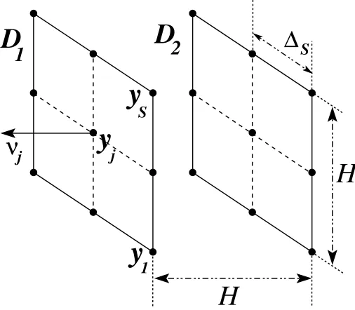
In order to identify relevant parameters for the accuracy of the equivalent sources, we give here a brief review of the two-face approach. Let us assume that true sources are embedded in a cube of edge sizeH

and generate a time-harmonic field with wave numberk. It has been established in [13, 14], and is also discussed in Appendix B, that there are equivalent sources on two opposite facesD1 and D2 of the cube

which approximate the initial wave to a high accuracy outside of a certain neighborhood of the source distributions.

In practice, these artificial point sources are constructed as follows: the two selected faces D1 and

D2 are each discretized using a set ofS×S equidistant nodes. This gives rise to two Cartesian uniform two-dimensional gridsτ_S(1) and τ_S(2) of mesh size ∆S =H/(S−1) which are located at the two faces D1

and D2, respectively, so there is a total of nS = 2×S×S such points. An equivalent monopole source ξj and an equivalent dipole sourceηj are placed at each nodey_j ∈τ_S(1)∪τ_S(2). The geometry is depicted

in Figure 3.1.

y

j

y

S

1

y

∆

S

ν

j

D

1 D

2 H

[image:32.612.178.431.378.599.2]

H

Figure 3.1: The two discretized faces in three dimensions

A second, larger cube also centered about the origin is constructed. We denote the union of its six faces by S_C _{and call it the collocation surface. Each face of this collocation cube is discretized into}

(33)

3.1 Parameter value identification 14

l∈ {1, . . . , nC}, where nC = 6×C×C−12×C+ 8 (see Section 3.1.1), the values of ξj =ξ(yj) and

η_j =η(y_j) forj ∈ {1, . . . , nS} are obtained by solving the overdetermined system

ˆ

u = h Am Ad i   ξ η 

, (3.1)

where the vector ˆuis defined by

ˆ u =             ˆ

u(x1)

.. .

ˆ

u(xl)

.. .

ˆ

u(xnC)

            , (3.2)

the monopole matrix is given by

{Am}_l,j = e

ikrl,j

4πrl,j, (3.3)

and the dipole matrix is

{Ad}l,j =

eikrl,j 4πr2_l,j

1

rl,j −ik

νj·rl,j. (3.4)

In (3.3) and (3.4), we use the notation rl,j = xl−yj, rl,j = |rl,j| and νj is the unit normal to the

two faces at y_j ∈ τ_S(1) ∪τ_S(2). The overdetermined system (3.1) is solved in the least-square sense by means of a singular value decomposition. The computational cost of this procedure is then an order

O(nC·n2S) operation. Hence, bothSandCshould be reasonably small, in order to avoid large computing

times. However, it should be noted that the singular value decomposition needs to be performed only

once. The equivalent sources evaluate then the field at any desired point outside of the collocation cell

by the matrix-vector multiplication (3.1). This algorithm is summarized in Appendix B.2.1. In the

(34)

the dependence of the algorithm’s performance on the values of the various associated parameters.

3.1.1 Accuracy as a function of collocation cube size

Le us consider a time-harmonic field with wave number k radiating from a point within a cubic cell ci

of side length H. On two opposite faces D1 and D2 of ci, an appropriate number of locations for the

equivalent sources nS = 2×_S×_S _{is selected (compare with Figure 3.1). We note that in [12, 13, 14],}

it is proposed to place the equivalent sources on the points of the extended planes ofD1 andD2 which

lie within the union of two circular domains concentric with (and containing) the faces ofci. The radius

of these domains is chosen to be equal to (or slightly larger than) half the length of the diagonals of

the faces. However, our finding is that in the context of the present work there is no disadvantage in

terms of accuracy and computing time if we choose to place equivalent sources directly on the Cartesian

grids τS(1) ∪τ (2)

S , and thus this shall be our standard choice in this thesis. We refer to Appendix B.2

for further discussion on this issue. We recall that in order to evaluate the equivalent sources, the field

needs to be specified at the nC = 6×_C×_C−₁₂×_C_{+ 8 collocation points of the surface} S_C_. _The

number nC results as sources are placed on each one of the six faces on the cube: on the first of the

three pairs of opposite faces, we place 2×_C×_C _{Cartesian points; on the second pair of opposite faces,}

only 2×_C×_C−₄×_C _{new positions can be located; and finally, on the last opposite pair, only the}

2×_C×_C−₈×_C_{+8 interior points of the Cartesian grid can be selected. We assume that the wave values}

at the collocation points along with the parametersk, H, S, C are known. The purpose of this subsection

is to determine the dimensions of a suitable collocation cube which is characterized by the edge length

HC. To this end, we select the specific values k= 10, S = 7, andC = 7 (which means thatnS = 98 and

nC = 218).Numerical results suggest it is best to choosenC at least 2nS.Numerical experiments further

indicate that under these constraints, any other choice of parameters for k, S, C lead quantitatively to

the same conclusions. We consider the five different values 2H,2.5H,3H,4H, and 5H forHC. Once the

collocation cube is known, Algorithm B.2.1 can be used to obtain an approximation of the wave at any

point outside of the collocation cube At the fixed point in space P = [0,1.25,1.26]t

, we compute the

numerical error EP(HC) to the exact solution in absolute norm. The results are displayed in Figure

3.2 for the four different values 0.00025,0.0025,0.025, and 0.25 for H. We note that the point P lies

outside of the collocation cube for all five choices ofHC. Figure 3.2 leads to the following observation:

(35)

10−4 10−3 10−2 10−1 100 101

10−10

10−9

10−8 10−7

10−6 10−5 10−4 10−3

H_C

E P

[image:35.612.124.485.82.366.2]

H=0.00025 H=0.0025 H=0.025 H=0.25

Figure 3.2: The errorEP(HC) as a function ofHC at P = [0,1.25,1.26]t

for different values of H

from the two facesD₁∪_D₂ _{to the collocation points} increases. _{Clearly, in this experiment the increased}

distance is realized by increasing the size ofHC while keeping H constant, and by doing so, the surface

S_C_{comes closer to the point}_P._{It might be thought that the decreased distance from}_P _{to the collocation}

points influences the conclusion “the bigger the collocation cube, the more accurate the equivalent source

computation.”

To see whether that is indeed the case, we consider the following experiment: for the valueH = 0.25,

we select one of the five parameters for HC from the first example, and we evaluate the error E(P) at

the location P = [0, l,0]t

, where l takes one of the nine values 0.6H,0.8H,1.2H,1.4H,1.5H,1.6H,2H,

or 3H.Clearly, the first point lies for all five collocation boxes between the surfaces of ci and SC, while

the last point is positioned outside the collocation cube. In Figure 3.3, we plot E(P) as a function of

P for the smallest and the largest collocation box, i.e., HC = 2H and HC = 5H, respectively. The

quantitative behavior is obvious: starting just outsideci and moving towardS_C_, _{the accuracy increases}

until the collocation surface is reached. Continuing moving in the same direction, the behavior remains

(36)

10−0.8 10−0.6 10−0.4 10−0.2 10−10

10−8 10−6

10−4 10−2

100

l

E(P)

[image:36.612.142.473.83.353.2]

H_C=2H H_C=5H

Figure 3.3: The errorE(P) as a function ofP = [0, l,0]t

for two different values of HC

experiment, we see that as the collocation cube increases, the more accurate the solution, despite the

fact that the point under consideration is closer. This leads to the conclusion that a larger collocation

box yields more accurate results.

As we will explain later, ideally, we want to choose HC as small as possible, but on the other hand,

the scheme should be as accurate as possible. These two trends conflict each other, and the selection

HC = 3H seems to be a reasonable compromise. Thus, HC = 3H is our standard choice if not stated

(37)

3.1.2 Point source at the origin

In this subsection, we assume that the point source ˜x of the Green’s function (A.12) is located at the

origin. The two facesD1 andD2 are centered about the origin, and given a certain wave number k and

side length H, we seek to determine the number of sources necessary to obtain a prescribed accuracy

from Algorithm B.2.1. The wave length is proportional to 1/k (see (A.9)), and therefore, ∆S should

be proportional to 1/k to adequately resolve the wave in space. Table 3.1 shows the accuracy of the

two-face approach for various parameters k, H, nS, and nC. The table is meant as an illustration only,

to demonstrate how the change of various parameters affects the accuracy of the solution. In the first

column, we consider four specific values for the wave number, i.e., k= 0,25,100, and 300. The value in

parentheses next to the wave number is its inverse, which gives a rough idea what the closest distance

between two equivalent sources is expected to be. Studies show that the biggest error to the exact

solution in absolute norm outside of the collocation box are found close to the surfaceS_C, _{as has been}

established in the last Section 3.1.1. In the second column, different sizes H of the panel length are

considered. The entries in the third, fourth, and fifth columns are all linked to the parameterS.To see

that the resolution of the equivalent sources lies in the right range, it is helpful to compare the closest

distance between the sources with the inverted values of the wave number. It is thus useful to consider

the value ∆S,which is given in the third column. The entries of the fourth column represent the number

of sources S along the panel-side H. The total amount of equivalent sources nS are tabulated in the

fifth column. These entries are helpful for estimating computing times. Similarly, the parameters ∆C, C

and nC are given in the sixth, seventh, and eighth columns, respectively. Finally, the values of the last

column correspond to the absolute error at the point [0,3H,0]t

.Table 3.1 shows that, as we expect, for

a fixedk and H, the accuracy increases as ∆S and ∆C are decreased. Interestingly, as we increase H

and keep the wave number k fixed, we can use larger ∆S and still obtain the same order of accuracy.

The number of sources, however, will generally increase as can be seen in Table 3.1 and also in Figure

3.5.

Now we pose the following question: given a wave number k and a panel lengthH, what mesh size

∆S is at least required to obtain a prescribed accuracy of the field? The answer can be found in Figures

3.4 and 3.5 for wave numbers up tok= 60 and panel lengths up toH = 0.5. The parameters are chosen

in such a way that the error in these figures is at least of the orderO₍₁₀−6

) outside of a sphere about the

(38)

k_{, (}1

k) H ∆S S nS ∆C C nC error

0, (∞) 0.025 0.0125 3 18 0.025 4 56 3·10−4

0.01875 5 98 1·10−5

0.0083333 4 32 0.01875 5 98 4·10−6

0.015 6 152 3·10−6

0.00625 5 50 0.01875 5 98 1·10−6

0.015 6 152 6·10−7

0.005 6 72 0.015 6 152 6·10−7

0.0041667 7 98 0.0125 7 218 8·10−9

0.0035714 8 128 0.0107143 8 296 3·10−9

0.075 0.025 4 32 0.05625 5 98 1·10−6

0.01875 5 50 0.05625 5 98 5·10−7

0.0125 7 98 0.0375 7 218 4·10−9

0.0107143 8 128 0.0321429 8 296 1·10−9

0.5 0.25 3 18 0.5 4 56 1·10−5

0.0833333 7 98 0.25 7 218 7·10−10

25, (0.₀₄₎ _0.025 _0.0125 ₃ ₁₈ _0.025 ₄ ₅₆ ₄·10−4

0.0083333 4 32 0.01875 5 98 1·10−5

0.00625 5 50 0.015 6 152 1·10−6

0.075 0.01875 5 50 0.05625 5 98 9·10−7

0.0107143 8 128 0.0321429 8 296 6·10−9

0.5 0.125 5 50 0.375 5 98 2·10−2

0.0833333 7 98 0.214286 8 296 2·10−4

0.0714286 8 128 0.214286 8 296 7·10−5

0.0625 9 162 0.1875 9 386 8·10−7

100, (0.₀₁₎ _0.025 _0.00625 ₅ ₅₀ _0.015 ₆ ₁₅₂ ₁·10−6

0.075 0.015 6 72 0.045 6 152 1·10−4

0.0375 7 218 2·10−5

0.0125 7 98 0.0125 8 296 9·10−7

300, (0._003333) _0.025 _0.0041667 ₇ ₉₈ _0.0125 ₇ ₂₁₈ ₄·10−6

0.075 0.00625 13 338 0.0160714 15 1178 8·10−7

Table 3.1: The field is generated by a point source located at the origin. The table demonstrates the

(39)

collocation points along the large cube of size 3H.If the accuracy fails to be achieved, it changesC up

to S+ 5, which means that there might be certain cases where the desired accuracy could be obtained

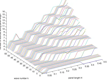
by choosing a lowerS and more thanS+ 5 collocation points. In Figure 3.4, we observe that in general, as k is held constant and H gradually increases, the mesh size ∆S can be chosen larger to obtain the

same accuracy of at leastO₍₁₀−6). But Figure 3.5 also reveals that “the larger H, the better” does not always hold. For k = 60 fixed, for example, we need to have only S = 4 sources along the panel length

H= 0.025, while it is required to haveS = 16 forH = 0.5. If we were to put equivalent sources on faces of the prescribed lengthH = 0.5, it would make more sense to partition them into a couple of panels of

(40)

0 5 10₁₅ 20 25 30₃₅ 40 45₅₀ 55

60 0 0.05 0.1

0.15 0.2 0.25 0.3

0.35 0.4 0.45 0.5 0 0.025 0.05 0.075 0.1 0.125 0.15 0.175 0.2 0.225 0.25

panel length H wave number k

mesh size

[image:40.612.115.491.80.361.2]

∆S

Figure 3.4: The mesh size ∆S as a function of the wave numberk and the panel lengthH to obtain at

least O₍₁₀−6) accuracy in the field values

0 5 10 15 20 25 30 35 40 45 50 55 0.05 0.1 0.15 0.2 0.25 0.3 0.35 0.4 0.45 0.5 3 4 5 6 7 8 9 10 11 12 13 14 15 16

number of sources along panel length

[image:40.612.119.495.413.693.2]

(41)

3.1.3 Point source at the most challenging location

Numerical experiments indicate that it is most challenging to position the test source ˜xat [H/2,0,−H/2],

or in the middle of one of the other three edges which connect the two faces D1 and D2. Table 3.2

dis-plays numerical accuracy for various parameter values. The structure of the table is the same as in

Table 3.1, but these two tables are not meant to directly compare with each other. Rather, Table 3.2

is supposed to demonstrate that high accuracy of orderO₍₁₀−7_{) for wave numbers up to} _k _{= 100 and}

panel lengths H between 0.01 and 0.05 can be achieved by selecting S and C in the range of 10 to

15. Computational results in [14] suggest that the accuracy increases by increasing kH, and the error

estimate (B.17) gives a rough order for the values considered there (kH = 8,12, and 16). Here, we are

interested in achieving a high accuracy for smaller values of kH. The results in Table 3.2 show that a

significantly higher accuracy can be achieved for small valueskHthan estimate (B.17) indicates. In fact,

Table 3.2 demonstrates that at least aO₍₁₀−7

) accuracy can be achieved forkH in the range of 0.25 to

5. For a given wave numberk and panel length H,the error is largely influenced by the choices of ∆S

and ∆C.The results fork = 100 in Table 3.2 suggest that for a fixed wave number, the accuracy indeed

increases with higherH: for the valuesH = 0.01 andH = 0.025 for example, the error ofO₍₁₀−7

) does

not improve asS andC are increased; forH= 0.05 however, the numerical approximation exceeds this

limit with appropriate values S and C.

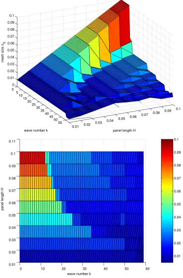
The diagrams in Figures 3.6 to 3.9 display the relationship that is needed between k, H, andS so that

the numerical solution approximates the true solution to at leastO₍₁₀−5₎_._{Figure 3.10 displays the}

num-ber of collocation points C used along one edge. The algorithm used here to determine the parameters

tests systematically forS fixed sources C=S and more collocation points until the desired accuracy is

achieved. If the desired accuracy fails to be reached for that number of sources, the algorithm increases

Sby one and the search for the lowest valueCstarts again. This is repeated until the appropriate values

S and C for a given k are found. The procedure is performed for all wave numbers of interest.

The rest of Chapter 3 deals with the extension of Algorithm B.2.1 to the time domain: time

de-pendent waves propagate from source distributions located inside of the cubic cell ci of edge length H

into the infinite three-dimensional space. The goal is to find time-dependent equivalent sources on the

faces D1 and D2 yielding a high-order representation of the field. At any point x∈ S_C, we imagine to

(42)

k H ∆S S nS ∆C C nC error

25 0.01 0.00111 10 200 0.00333 10 488 1·10− 8

0.000909 12 288 0.002727 12 728 2_·10−7 0.000714 15 450 0.001875 17 1538 2·10−

7

0.025 0.00277 10 200 0.00833 10 488 2·10− 8

0.00227 12 288 0.006818 12 728 5_·10−8 0.05 0.00556 10 200 0.01667 10 488 2·10−

8

0.004545 12 288 0.013636 12 728 4·10− 8

50 0.01 0.00111 10 200 0.00333 10 488 1·10− 8

0.000909 12 288 0.002727 12 728 1·10− 7

0.000714 15 450 0.001875 17 1538 2_·10−7 0.025 0.00277 10 200 0.00833 10 488 4·10−

8

0.00227 12 288 0.006818 12 728 9·10− 8

0.05 0.00455 10 200 0.01667 10 488 9_·10−8 0.004545 12 288 0.01363 12 728 2·10−

7

75 0.01 0.001111 10 200 0.0033333 10 488 9·10− 7

0.000909 12 288 0.0027273 12 728 2·10− 7

0.000714 15 450 0.001875 17 1538 3_·10−7 0.025 0.002778 10 200 0.0083333 10 488 8·10−

8

0.002273 12 288 0.0068182 12 728 1·10− 7

0.001786 15 450 0.0046875 17 1538 2_·10−7 0.05 0.005556 10 200 0.0166667 10 488 4·10−

7

0.004545 12 288 0.0136364 12 728 3·10− 7

0.003571 15 450 0.009375 17 1538 2_·10−7 0.075 0.008333 10 200 0.025 10 488 2·10−

6

0.006818 12 288 0.0204545 12 728 3·10− 7

0.005357 15 450 0.0140625 17 1538 2_·10−7 100 0.01 0.00111 10 200 0.00333 10 488 1·10−

6

0.000909 12 288 0.002727 12 728 3_·10−7 0.000714 15 450 0.001875 17 1538 3·10−

7

0.025 0.002778 10 200 0.008333 10 488 2·10− 7

0.002272 12 288 0.006818 12 728 4·10− 7

0.001786 15 450 0.004688 17 1538 4·10− 7

0.05 0.005556 10 200 0.016667 10 488 1_·10−6 0.004545 12 288 0.013636 12 728 4·10−

7

[image:42.612.139.472.140.635.2]

0.003571 15 450 0.009375 17 1538 2·10− 8

(43)

0 5

10 15

20 25

30 35

40 45

50 55

0.01 0.02

0.03 0.04

0.05 0.06

0.07 0.08

0.09 0.1 0

0.01 0.02 0.03 0.04 0.05 0.06 0.07 0.08 0.09 0.1

mesh size

∆S

0 10 20 30 40 50 60

0.01 0.02 0.03 0.04 0.05 0.06 0.07 0.08 0.09 0.1 0.11

wave number k

panel length H

[image:43.612.122.491.105.666.2]

0.01 0.02 0.03 0.04 0.05 0.06 0.07 0.08 0.09 0.1

Figure 3.6: Hardest case: The mesh size ∆S in relation to the wave numberk _{and the panel length}H

(44)

0 5

10 15

20 25

30 35

40 45

50 55

0.01 0.02 0.03 0.04 0.05 0.06 0.07 0.08 0.09 0.1

2 3 4 5 6 7 8 9 10 11

wave number k panel length H

[image:44.612.123.487.85.361.2]

number of sources along H

Figure 3.7: Hardest case: The number of equivalent sourcesS _{along one panel length in dependence of}

the wave numberk _{and the panel length}H _{to obtain at least} O₍₁₀−5) accuracy in the field values

0 5 10

15 20 25

30 35 40

45 50 55

0.01 0.02 0.03 0.04 0.05 0.06 0.07 0.08 0.09 0.1

2 3 4 5 6 7 8 9 10 11

Figure 3.8: Hardest case: The number of equivalent sourcesS _{along one panel length in dependence of}

[image:44.612.122.485.419.690.2]

(45)

0 5 10

15 20 25

30 35 40

45 50 55 0.01

0.02 0.03 0.04 0.05 0.06 0.07 0.08 0.09 0.1

2 3 4 5 6 7 8 9 10 11

0 10 20 30 40 50 60

0.01 0.02 0.03 0.04 0.05 0.06 0.07 0.08 0.09 0.1 0.11

wave number k

panel length H

2 3 4 5 6 7 8 9 10 11

(46)

0 5 10

15 20 25

30 35 40

45 50 55

0.01 0.02 0.03 0.04 0.05 0.06 0.07 0.08 0.09 0.1

4 5 6 7 8 9 10 11 12 13 14

number of collocation points

0 10 20 30 40 50 60

0.01 0.02 0.03 0.04 0.05 0.06 0.07 0.08 0.09 0.1 0.11

wave number k

panel length H

4 5 6 7 8 9 10 11 12 13 14

(47)

for details). We associate the collocation surface with the Kirchhoff surface, and, in view of Kirchhoff’s

formula, the partition of the solution of the wave equations can be evaluated packetwise at any point

outside ofS_C _{before adding the packets by superposition principle to the wave function together.}

There-fore, it is natural to develop and study the concept of the equivalent sources for time-periodic waves first,

which we do in the next section. The interest of this discussion is mainly theoretical, however, since,

as mentioned in Section 3.3.1, an alternative approach introduced in Section 3.3, based on a certain

“continuation method” for Fourier series, can be significantly more efficient in practice.

We close this section with a final remark. Let us assume that a time dependent wave is propagating

from a point source into the open three-dimensional space. The point source is located in ci between

the faces D1 and D2. In view of equation (2.1), this means that the forcing term takes the form

f(x, t) = 4πδ(x−x0)s(t), (3.5)

where x0 is the position of the point source and s(t) is an arbitrarily, sufficiently smooth function

representing the strength of the source at timet. We recall that the Kirchhoff representation (2.6) solves

(2.1). Since the problem is purely outgoing from a point source into the three-dimensional space, the

surface integrals (2.8) and (2.9) vanish and the solution (2.6) simplifies to

u(x, t) = Z

R3

f(˜x, t−r/c)

4πr dx˜ =

s(t−_r/c₎

r , (3.6)

wherer is the distance fromxto the location of the sourcex0. This simple model enables us to evaluate

the exact solution to the wave equation very easily without any numerical integration rules. Under the

assumption that the field is known on the collocation surface S_C, _{our goal is to compute an equivalent}

source distribution on the two facesD1andD2, which represents the wave outside ofSC.This is discussed

in subsequent sections.

We note that this point source solution can also be used to construct a simple solution to the more

complicated case when a scatterer is present: we place a fictitious point source inside _{the scatterer.}

We know that (3.6) solves the wave equation; thus, if we impose on the scatterer’s surface a boundary

condition that assumes the form (3.6) for the field values, the exact solution to the problem (2.1)–(2.5)

(48)

3.2 The time-dependent periodic case

In this section we assume that the continuous wave functionu(x, t) is T-periodic at any pointxoutside

of ci, i.e., u(x, t) =u(x, t+T). Thus, forx∈R3\c_i, the field can be expanded by the Fourier series

u(x, t) = ∞ X

n=−∞

ˆ

un(x)e 2πi

T nt, (3.7)

with the Fourier coefficients

ˆ

un(x) = 1

T

Z T

0

u(x, t)e− 2πi

T ntdt. (3.8)

Substituting (3.7) into the homogeneous wave equation, multiplying by e−2πimt/T and integrating over

the time domain [0, T] leads to the Helmholtz equations

∆ˆun+k2nuˆn = 0, for x∈R3\c_i, (3.9)

where the wave numbers are defined as

kn = 2π

cTn. (3.10)

In view of the two-face approach, it is clear that monopole equivalent sourcesξn(l) and dipole equivalent

sourcesηn(l) can be found on the two discsDl for each frequency indexn.The Fourier coefficients ˆunare

thus represented to high-order accuracy by the corresponding frequency-dependent equivalent sources.

Under the assumption that the Fourier coefficients of the considered waves are rapidly converging to zero

as|n|increases, only few frequency modes need to be considered to achieve a very accurate approximation

of (3.7). We summarize the procedure in

Algorithm 3.2.1.

1. Transform the given data u(x, t_m) at the collocation points x∈ S_C into the Fourier space which

gives ˆun(x) for {m, n} ∈ {0, . . . , N−1}.

2. Apply Algorithm B.2.1 to theN Fourier coefficient. This results in the equivalent sourcesξn(l)∪η(nl)

(49)

3.2 The time-dependent periodic case 30

3. Algorithm B.5.1 can now be applied to evaluate ˆun(x) on any Cartesian grid τ(3)

F outside of SC

fast (see Appendix B for details).

4. The inverse Fourier transform in time atx∈τ(3)

F gives the approximation tou(x, tm).

3.2.1 Numerical example

As an example, let us assume that the propagation velocity is c= 1 and take s(t) (see equation (3.5)) to equal the Gaussian function

s(t) = e−(t−t0)2/σ2

, (3.11)

with σ = 0.4 and t0 = 3. The function’s values outside the interval 0 ≤ t ≤ 6 are no larger than

O(10−₂₅

), and thus repeating this function periodically with period 6 gives rise to a discretization of a

periodic smooth function of periodT = 6 up to rounding errors. The function and its discrete Fourier transform withN = 32 points are plotted in Figure 3.11. Applying the inverse Fourier transform to the Fourier coefficients {sˆm}Nm=0−1 gives the approximated values at the N points. The maximum absolute error at these points to the original function s(t) is 3·10−₆

. To determine how well the N frequencies approximate the function at other points, we can extend the Fourier spectrum by zero padding, i.e., the

modified Fourier coefficients {s˜m}Nm˜=0−1 take the form

˜

sm =

     

    

ˆ

sm, ifm∈ {0, . . . , N/2} ,

ˆ

s_N−_N˜₊_m, ifm∈ {N˜ −1, . . . ,N˜−N/2 + 1} , 0, otherwise.

(3.12)

In (3.12) we assume that Ñ = 2αN, where α is a positive integer. Applying an inverse Fourier trans-form to the zero-padded coefficients samples the approximated function at Ñ equidistant points in the physical time domain. The two lower pictures of Figure 3.11 illustrate this for Ñ = 2N. For a fixed

(50)

0 1 2 3 4 5 6 0

0.2 0.4 0.6 0.8 1

time

s(t)

Gaussian Function

0 5 10 15 20 25 30

−4 −2 0 2 4

frequency

real part

0 10 20 30 40 50 60

−4 −2 0 2 4

Zero padding

frequency

real part

0 1 2 3 4 5 6

0 0.2 0.4 0.6 0.8 1

time

s(t)

Nonreflecting boundary conditions obtained from equivalent sources for time dependent scattering problems