A
STUDY
OF
TSUNAMI
MODEL
FOR
PROPAGATION
OF
OCEANIC
WAVES
1
E.SYED MOHAMED, 2 S.RAJASEKARAN
1
Department of Computer Science and Engineering BS Abdur Rahman University, Chennai,INDIA
2 Department of Mathematics
BS Abdur Rahman University, Chennai, INDIA
E-mail: [email protected], [email protected]
ABSTRACT
The enormous destruction of tsunami and the increased risk of their frequent occurrences enhance the need for the use of more sturdy and accurate models that predict the spread of catastrophic oceanic waves accurately. This paper tries to study this phenomenon that shows a considerable amount of uncertainty. To model the spread of tsunami waves, the initial wave can be considered as a continuous two dimensional closed curve. Each point in its parametric representation on the curve will act as a point source which expands as a small ellipse. The parameters of each ellipse depend on many factors such as the energy focusing effect, travel path of the waves, coastal configuration, offshore bathymetry and the time step. Using Huygens’ wavelet principle, the envelope of these ellipses describes the new perimeter. Further, overlapping and traversing of the wave front are detached and efficiently clipped out
Keywords: Huygens’ Wavelet, Tsunami Propagation, Simulation, Curvature, Convex
1. INTRODUCTION
The damage of properties and loss of lives by tsunamis highlight the need for real-time simulation systems accurately predicting their spread. In order to combat this natural hazard, the scientists have used numerous models to predict the propagation of oceanic waves. These are used in the computer-based decision support system that incorporates real-time assimilation of the phenomenon by prompt and expeditious collection of data from various sources. By utilizing different spread algorithms prompt warnings may be issued for a program of preparedness. These will be used as a real time tsunami warning system for controlling disasters.
The aim of this paper is to provide a graphical representation of the development of tsunami waves that spread under spatially variable topographic, slope and meteorological conditions. The development of a suitable planning and allocation of resources is a critical phase in mitigating tsunamis. This can be enhanced by reliable simulations of the propagation of a reported tsunami, spreading under actual or forecast conditions. Constantin et al[1] discussed the range
of validity of nonlinear dispersive integral equation for the modeling of propagation of tsunami waves. By considering a three layer system, the generalized governing equations for multilayered long wave system was developed by Imteaz et
al[2].Recently, Marchuk [4] investigated
numerically the tsunami wave behavior above the ocean bottom ridges using finite difference method. Prasad Kumar et al [5] used the Huygens’ method for computing the tsunami travel times for Indian ocean based on isochrones table. Lehfeldt et al[3] studied the propagation of a tsunami wave in the north sea by performing numerical simulations and found out the most affected areas in the north sea and the German bight.
ISSN: 1992-8645 www.jatit.org E-ISSN: 1817-3195
This emphasizes that developing a better
understanding of the spread of the sections of the perimeter is essential for models of tsunami perimeter spread across the ocean under various cases [12].
2. GEOMETRICAL EXPANSION
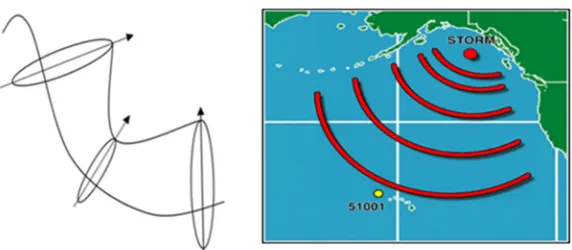
According to Huygens’ Principle, every point on the wave front will produce another wave front. Both straight lines and circular waves are propagated using Huygens’ Principle. Waves travelling in a ocean or lake also follow Huygens’ principle. The new wave front can be derived from Huygens’ Principle as follows: From the epicenter the position of the wave front can be evaluated in all directions after particular interval the correction of the positions will give the wave position at that time. The points at that position become the new sources for the wave from which the positions are evaluated for the next time interval (Figures 1-3).
A simple geometric model, based on Huygens’ principle, incorporating elliptical spread at each point on the wave front, is proposed .We assume that each point on the wave front at time t expands
as a small ellipse. The new wave front at time t +∆t
is defined as the outer envelope formed by small ellipses (Figure 4).
The propagation ellipse at each point can be
expressed in form
(
)
12 2 2 2 = + − b y a c
x where the
forward, flank and back rates of spread are defined
as
(
)
t b t c a ∆ ∆ +
, and
(
)
t c a
∆
− respectively.
If we limit c as per like constraint a²=b²+ c², the focus of the propagation ellipse and the origin of the coordinate system coincide with the point on the old perimeter. In this form, the wave direction is aligned with the x-axis. The ellipse parameters for each point on a wave front can be estimated from the forward rate of spread and other parameters. There are two critical assumptions in this application of Huygens’ Principle. It is assumed that each point propagates independently of its neighbors as a small ellipse with the ellipse parameters only dependent on how the energy is focused, the travel path of the waves, the coastal configuration and the offshore topography. Further, it is assumed that the spatial variables which effect rate of spread are constant beneath the whole ellipse
for the period ∆t. Hence, errors will be minimized
as ∆t 0 and as number of points tend to ∞.The
purpose of the algorithm described in this paper is to define the envelope in a speedy and precise manner. The algorithm is presented as follows.
3 ALGORITHM DESCRIPTIONS
The method of perimeter expansion algorithm is based on determining points on the new perimeter. The wave front (perimeter) is
maintained as a set of points Wt, in clockwise
order. The algorithm first accesses the database for
information at each point Pt,i in the perimeter Wt .
Parameters such as energy, travel path, coastal configuration are used for the selected rate of spread at each old perimeter point. We define the ellipse parameters a, b, c using the estimated forward rate of spread and the length to breadth ratio. A point or points on the propagating ellipse are then selected for inclusion in the new perimeter
Wt+∆t.
At each old point, we define the deflection, D as line change of direction of the old perimeter such that a point in a concave part of the perimeter has a negative deflection. We define four curvature categories accordingly to the deflection, D, at the point on the old perimeter.
Concave when 4 π − ≤ D
Low curvature when
4 4
π π < <
−
D
Moderately convex when
2 4
π
π
≤ ≤D
Sharply convex when
2
π
>
D
If a point on the old perimeter is on the section of perimeter of low curvature we select only one point on the propagating ellipse to contribute. if sharply convex we identify three points on the perimeter and in the case of moderately convex points and concave points we identify two points on the perimeter of the propagating ellipse for inclusion. To identify these points we use some additional concepts on ellipse.
The locus of the ellipse with respect to the old perimeter point, can be represented in the parametric form
θ
θ
θ
θ
θ
θ
sin cos sin cos sin cos cos cos sin sin S a C S b Y S a C S b X − − = − += -- (1)
where
θ
is the angle of the wave direction and thegradient at any point on an ellipse can be expressed in terms of the parametric variable, S.
dx dS dS dy dx dy
Gradient = = .
Thus, for some gradient G, the required value of the parameter S is given by
− − = − ) sin cos G ( a ) cos sin G ( b tan S θ θ θ θ 1
There are two solutions for S in [0,2ߨ].So,
given a gradient, the coordinates of two tangent points can be determined using (1).The two tangent points p1 and p2 are on the opposite sides of the ellipse. Here we are only interested in the tangent toward the outside of the old perimeter.
Using vector algebra, for a given vector u,
we can identify two points p1 and p2 on an ellipse
such that the gradient of the ellipse at those two points are equal to the gradient of the vector. We
define the outward normal n, by rotating the vector
u by
2
π
radians in an anticlockwise direction
(Figure 5).
The scalar product of the vector joining the focus and the point p1 with the outward normal is greater than 0, so p1 is the required tangent point. So, given a vector or its gradient, we can identify which of the tangent points on the propagation ellipse is toward the outside of the old perimeter.
4. OVERLAP DETECTION AND REMOVAL
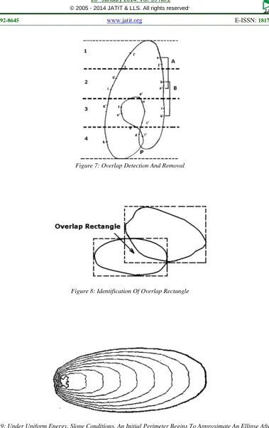
If a section of perimeter is affected by an area of low spread, the advancing perimeters either side of that area can eventually overlap (Figure 6)
Our interest is in the external perimeter of the waves, rather than the internal untraversed area which may or may not be eventually traversed. The easy approach would be to check every line for an intersection with every other line, a tedious but possible for computer task.
Otherwise, we divide the perimeter into segments. Segments are defined by a division of the wave front into equal horizontal zones (Figure 7).
A segment is defined as all the points in a length of perimeter as it crosses a zone. The first and last point in a segment actually resides in the adjacent zones.
Each segment is compared against each other segment, except for itself and adjacent segments which by definition can provide no intersections. In the figure the perimeter is divided into four zones and has ten segments. Segment A includes all points from point a to a’. Similarly, B includes all points from b to b’ etc, Although segments B and D,B and E, and B and H share the same zone numbers, their maximum and minimum x values do not overlap, hence no line intersections can exist. Segments C and G share the same zone numbers and their maximum and minimum x values do overlap so we check for intersections between the line segments. An overlap which occurs completely within one zone may persist until it grows large enough to spread across more than one zone.
5. MERGING OF PERIMETERS
A related task in the system with multiple wave fronts is the merging of two different perimeters. If more than one wave front is being propagated then a rectangle aligned with the coordinate system which just spans the perimeter is formed. If rectangle associated with separate perimeters overlap then we can define overlap rectangle (Figure 8).
A line of intersection check is performed to identify the intersection points. If any are found the two perimeters are merged by clipping out those points between the intersection points. The intersection point P is identified and the internal loops clipped out of the perimeter. Even though C and F intersect, the loop is an inside loop within the point of intersection P of C and G.
6. VALIDITY OF THE MODEL
Our model can be validated by considering the simulation of tsunami waves under different cases. When the initiating wave has a small irregular perimeter, the algorithm produces a large elliptical wave front under uniform energy conditions as is commonly observed (Figure 9).
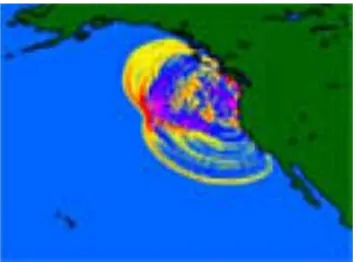
The spread of the algorithm is satisfactory when predicting wave spread which is occurring on a scale of seconds under homogeneous and non-homogeneous oceans (Figure10).
The results obtained by our model are in commensuration with the tsunami data available
ISSN: 1992-8645 www.jatit.org E-ISSN: 1817-3195
tsunami of 2007 and wave propagation from 1700 Cascadia tsunami developed by geological survey of Canada(Figures11-12).
With a simple geographical database consisting of one large polygon of ocean with high tsunami danger and uniform energy type, a single point explosion developed into an elliptical perimeter. When the density of points on a part of the perimeter becomes sparse we can add intermediate points, thus increasing the number of points in defining the perimeter.
6.1 Tsunami N2 model to understand tsunami Wave propagation in Indian Ocean after
26thDecember, 2004 earthquake
The model has been validated from the observed tide gauge wave amplitude from the ports on 26th December, 2004. The following figures show the relationship between the derived wave amplitude and observed tide gauge measurement at the four sites using ETOPO5 and ETOPO2 bathymetry.
Propagation states at t = 5, 30, 60, 90, 120, 180, 190 and 300 minutes (Figures 13-14)
7. LIMITATIONS FOR IMPLEMENTATION
With the inaccuracy related to the models used to generate the propagating ellipses, the
application of Huygens’ Principle to the
propagation of wave fronts rests on two
assumptions. That is points propagate
independently of their neighbors and that rate of spread varies linearly between adjacent points. Moreover, the spatial variables effecting rate of
spread are constant for the period ∆t.
The performance of this algorithm in defining the enveloping curve is also limited by the assumption made regarding the location and number of points on each propagating ellipse that are included in the new wave front. The ideal enveloping curve would consist entirely of the common tangents between neighboring propagating ellipses connected with arcs from the ellipses. We use the gradient of the old perimeter. That gradient is only equal to that of the common tangent between the ellipses if the ellipses are identical. Hence the tangent points we derive only approximate the true tangent points. In some cases we may have to use iteration method to determine the tangent points. The magnitude of the errors associated with the enveloping curve approximation are trivial that are inherent in the practical
application of Huygens’ Principle to the
propagation of a wave front.
8. CONCLUSIONS
We have described an algorithm based on Huygens’ frontal propagation in an explicit manner. Points on the perimeter of propagating ellipses are selected to form a new perimeter which approximates the ideal enveloping curve. Each newly defined perimeter is corrected to remove rotations which are generated at concave points. Further the overlapping sections of the perimeter are identified efficiently and any internal loops, if any, formed are clipped out of the perimeter leaving only the outer perimeter which is of principal interest. The algorithm is fast enough to be useful in real time simulation of the spread of tsunami waves.
REFERENCES:
[1].
Adrian Constantin (2009), ”On the propagationof tsunami waves, with emphasis on the tsunami of 2004”, Discrete and continuous
dynamical system series B 12(3)2009,525-537
[2].
Imteaz M.A., F.Imamura, J. Nazer(2009),”Governing equations for multilayered tsunami waves”, Science of Tsunami Hazards 28(3)2009,179-185
[3].
Lehfeldt R., ,P.Millradt , A.Pluss andH.Shiittrumpf “Propagation of a tsunami-wave
in the north sea” www.bauinf.uni-hannover.de/
[4].
Marchuk A.G.,(2009), “Tsunami wavepropagation along wave guides”, Science of
Tsunami Hazards,28(5) 2009,283-302
[5].
Prasad kumar B,R Rajesh kumar,S.K.DubeTad Murty,Avijit Gangopadhyay,Ayan
Chaudhri and A.D.Rao(2006),”Tsunami travel time computation and skill assessment for the 2O6 December 2004 event in the Indian
Ocean”, Coastal Engineering Journal
48(2),2006,147-166
[6].
http://iisee.kenken.go.jp/special/fujii_Solomon_ HP/tsunami.html[7].
Wessel,Geoware,http://www.geoware-online.com[8].
http://www.iirs-nrsc.gov.in/annual_report_2005-06.pdf[9].
Boudewijn Ambrosius, Remko Scharroo,Simons,”The 26th December 2004 Sumatra Earthquake and Tsunami Seen by Satellite Altimeter and GPS”. Geo-information for
Disaster Management Journal (2005),323-336,
XXVI, 1434 p. 516 illus., Hardcover,ISBN: 978-3-540-24988-7
[10]. Annunziato.A ” Development and
Implementation of a Tsunami Wave
Propagation Model at JRC”. Proceedings
of the International Symposium on Ocean Wave Measurement and Analysis. Fifth International Symposium on Ocean Wave Measurement and Analysis.
Madrid 3-7 July 2005
[11]. Annunziato,A “The Tsunami assessment modeling system by the joint research centre”,The International Journal of The
Tsunami Society, vol 26(2), 2007,p 70-9
[12]. S.Rajasekaran and E.Syed Mohamed , “A
geometric model for propagation of tsunami
waves”, Proceedings of 4th International
Tsunami Symposium, July 25- 29, 2010,
ISSN: 1992-8645 www.jatit.org E-ISSN: 1817-3195
[image:6.612.98.505.68.270.2]
Figure 1: Propagation Of Waves In Different Cases
Figure 2: New Wave Front By Huygens’ Principle
[image:6.612.171.457.550.675.2][image:7.612.89.523.71.293.2]
Figure 4: Application Of Huygens’ Principle
Figure 5: Selection Of The Outside Tangent Point
[image:7.612.208.404.537.656.2]ISSN: 1992-8645 www.jatit.org E-ISSN: 1817-3195
[image:8.612.201.419.338.447.2]
Figure 7: Overlap Detection And Removal
Figure 8: Identification Of Overlap Rectangle
[image:8.612.198.417.541.636.2][image:9.612.238.418.303.455.2]
Figure 10: The Performance Of The Algorithm Under Homogeneous And Non-Homogeneous Cases.
Figure 11: Solomon Island Tsunami On 2007/4/1 [6]
[image:9.612.240.418.513.644.2]ISSN: 1992-8645 www.jatit.org E-ISSN: 1817-3195
Figure 13: Tsunami Propagation States In The Indian Ocean With Tsunami N2 Simulation Model
Figure 14: The 26 December 2004 Tsunami Seen By The JASON-1 Altimeter Jointly Operated By NASA And CNES. The Map Shows The Modeled Tsunami And Satellite Track Along Which Altimeter Data Was Used To Obtain Sea Level
[image:10.612.207.413.406.552.2]