A MULTI-STEP PREDICTION MODEL BASED ON
INTERPOLATION AND ADAPTIVE TIME DELAY NEURAL
NETWORK FOR TIME SERIES
1LIANG GAO, 2YIHUA ZHANG, 3MENG ZHANG, 4*LIMIN SHAO, 4JINGXIN XIE
1
Administration Department of science and Technology, Hebei Agricultural University, Baoding 071001, China
2Jibei Baoding Electric Power VOC. & TECH. College, Baoding, 071051, China
3College of Information and Electrical Engineering, China Agricultural University, Beijing 100083, China
4College of Mechanical and Electrical Engineering, Hebei Agricultural University, Baoding 071001, China
*Corresponding author: [email protected]
ABSTRACT
The drawback of indirect multi-step-ahead prediction is error accumulation. In order to tackle this problem and improve the capacity of adaptive time delay neural network (ATNN) for prediction, a three-stage prediction model SATNN based on spline interpolation and ATNN is presented. With spline interpolation and ATNN, the impact of last prediction errors that would be iterated into the model for the next step prediction is decreased, and then the better prediction can be obtained. The annual sunspot, considered as the benchmark chaotic nonlinear systems, is selected to test the multi-step prediction model. Validation studies indicate that the proposed model is quite effective in multi-step prediction.
Keywords: Multi-step Prediction, Time Delay, Adaptive Time Delay Neural Network, Spline Interpolation
1. INTRODUCTION
Multi-step prediction is a kind of typical prediction algorithm, it obtained in consecutive predicted value of multiple time points based on the previous measurement data. However, with the existing method to realize multi-step prediction, when the forward one step prediction, the input data of neural network model for forecasting is a number of observed values before the time point of prediction, and as the prediction step increase, the last input of previous predictive values increased gradually, resulting in deterioration of prediction results.
There are many literatures were documented as the neural network for multi-step prediction [1-18], but most of the algorithms are too complex, and their running time is very long. Especially working with large amounts of data, the convergence speed is slow, and the prediction accuracy is not very high. Among them, the recurrent neural network has been proved to be an effective method of multi-step prediction, but it required for a long time for the training, and the robustness is poor, so it brings certain difficulty to the implement.
In addition, time delay neural network (TDNN) and its improved model adaptive time delay neural
2. THE MODEL AND THE ALGORITHM
2.1The Model Architecture
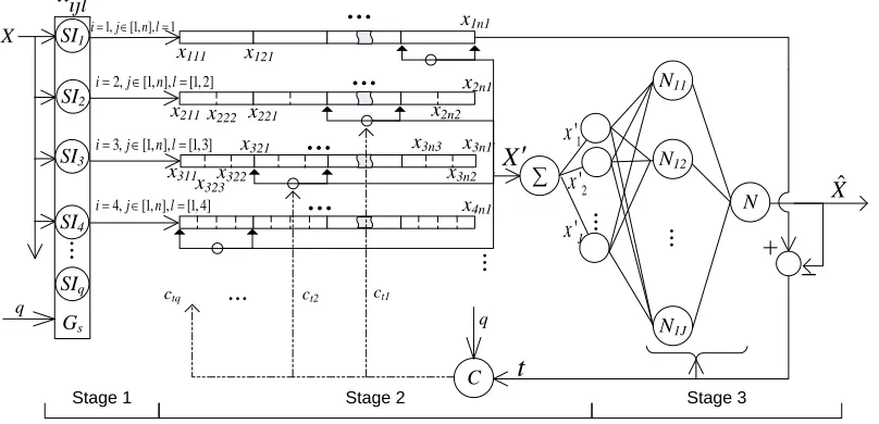
The model architecture and algorithm diagram was
shown in Figure 1. The first stage
G
s is thegenerator of spline interpolation unit; it could
[image:2.612.108.512.182.377.2]produce a number of virtual sequences; the second stage, a certain proportion data were extracted from the output sequence of the interpolation units, to form a new sequence; stage third, the use of ATNN on the new sequence forecast.
Figure 1: The Three-Stage Architecture Of Prediction Model SATNN
2.2 Algorithm
In the first stage, different interpolation unit, using different sampling frequency, inserted the smoothing data in the original. Set D as the original sampling frequency, using third-order piecewise polynomial functions, then the B-spline interpolation could be described as
∑ = − ′ = ′ n k k k k c k S 1 ) ( 3 ) ( 3 ) ( 3 β (1)
Where
[ ]
−
∈
∈
′
r
q
r
r
r
r
k
1
,
2
,
,
1
2
,
,)
(
)
(
0 0 0 03
x
β
β
β
β
x
β
=
∗
∗
∗
,
−
≤
≤
=
otherwise
x
x
,
0
2
1
2
1
,
1
)
(
0β
,k
′
is theinterpolation points,
n
is the length of original sequence, operator∗
denotes convolution, andq
is the number of B-spline interpolation units.When the model in prediction of forward
p
point (
x
ˆ
t p+ ), ifp
>
1
, the predictive value is moreand more dependent on the previous predictive, so using the interpolation method, in the second stage, a sequence
X
′
is derived out from the originaldata dynamically. The sequence can be expressed as
=
=
=
=
+ − + − − − − q q t q J t t t t t t tx
x
x
x
x
x
x
x
) 1 ( 1 2 2 2 1 2 1 1 1 0'
,
,
'
,
'
'
(2) Where2
)
1
(
+
=
q
q
J
,t
∈
[
p
+
1
,
n
]
,t
represents the current time,
J
is the sequence length.As a result of model training needs,
t
interval ist
∈
[
p
+
1
,
n
]
. Whent
is different,X
'
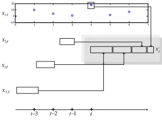
is a dynamic sequence. After the interpolation and dynamic combination, the time series of original data have lost its meaning. In the next stage of model, it mainly focuses on the serial number of sequenceX
'
. Figure 2 shows the diagram of the interpolation and dynamic combination (takeq
=
4
).Based on the first two stages, the multi-step prediction can be shown as
)
'
ˆ
,
,
'
ˆ
,
'
ˆ
(
'
ˆ
t+p=
F
x
t+p−1x
t+p−2x
t+p−τx
(3)...
...
…
…
…
…
...
...
+
_
...
Stage 1 Stage 2 Stage 3
x1n1
x111 x121
Gs N X ct1 x211 ijl
x
'
Jx
2, [1, ], [1, 2]
i= j∈ n l=
1, [1, ], 1
i= ∈j n l=
3, [1, ], [1,3]
i= j∈ n l=
4, [1, ], [1, 4]
i= j∈ n l=
x222 x221
x2n1
Where
0
≤
τ
≤
J
−
1
, the variables with "^" express the predictive value. In the third stage, thelth layer of ATNN has
N
Lneurons, the input and output matching for adaptive neuron is shown as(
)
1
( ) 0 1
M
i i i i
i
y t σ ωx t τ τ J
=
= − ≤ ≤ −
∑
(4)
Where the weight of the neuron is
ω
i,i
τ
is time delay and σ( )⋅ means nonlinear activation function. Then, the prediction model with one hidden layer is expressed as)
(
)
(
1
1
1 l
ji N
i l i l ji j
l
t
o
w
t
net
l
τ
−
=
∑
−
=
−
(5)
Where
0
≤
τ
lji≤
J
−
1
,o
(
t
)
(
net
j(
t
)
)
l l lj
=
σ
,the output of the jth neuron of the lth layer is
recorded as
o
lj(t
)
. Such as{
( )
}
1
| ,0 1
i
o t xt i′− ≤ ≤ −i J is
the output of the ith neuron of the first layer, and
1
1
ˆ
ˆ
t′
+=
x
t+x
is the predictive value ofx
i+1.3. EXPERIMENTS AND DISCUSSION
In order to verify the model's validity, the experiment tested by the benchmark time series, average numbers of annual sunspots. The sequence is a famous example of international statistics field, is the touchstone of testing a variety of modeling methods [5, 6, 19]. In this work, it chose the Wolfer Sunspotss data sets as the testing content. In order
to compare with other literatures, selection the sunspot data from 1700 to 1920 as the training sets, 1921 ~ 1954 and 1955 ~ 1979 as the testing sets, are expressed as Set1 and Set2 respectively. Using standard mean square error measures the predicted results.
The ATNN topology of the third stage is a three layers BP network containing one hidden layer, its design parameters as follows: maximum delay is 4, in order to make the expanded data sequence also
keeping this delay, so
τ
max=
10
, then the inputnode points of ATNN is 10 [20, 21]. The node number of hidden layer can be obtained by experiment (take as 13).
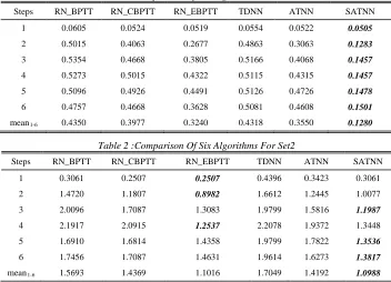
[image:3.612.240.407.469.593.2]In order to verify the validity of SATNN, 40 experiments were conducted for Set1 and Set2 respectively and averaged, for considerations of simplicity and accuracy, using only the existing literature data and the model for comparison, without these model simulations. In addition, this work also simulated with the similar model of TDNN and ATNN. Table 1 is the model for Set1 prediction error and other model simulation results, RN_BPTT, RN_CBPTT and RN_ECBPT are based on recurrent neural network model, the results were come from the literature [2]. It can be seen that this model performed best in the above 6 models, the minimum prediction error is marked out by bold italic.
Figure 2: Sequences From The Second Stage
Table 2 is the model for Set2 prediction error and other model results. It can be seen that, in the above 6 models, the model is most close with the RN_ECBPTT, when step was 1, 2 and 4 RN_ECBPTT error is minimum, step 3, 5 and 6 SATNN error is minimized, and the 1~6 step prediction error of the mean value is the minimum.
Therefore, through the transform of data interpolation, it improves the ATNN multi-step predictive ability effectively, but also with a relatively simple network structure to achieve recursive neural network prediction.
0 1 2 3 4 5 6 7
-10 0 10 20
Xt′
1jl X
2jl
X
4jl X
3jl
X
t + + + +
1
t−
2
t−
3
4. CONCLUSION
With the inspiration of spline interpolation, time delay and dynamic time delay neural network, this manuscript presents a combined three stage multi-step prediction model. In the first stage, through multiple interpolation units generate an interpolation sequence of different number; the second stage, from multiple interpolation sequence derived from a new sequence in dynamic; the final stage, the adaptive time delay neural network completed the prediction. The tested results of the
[image:4.612.129.481.247.501.2]two benchmark time series show that, the model in multi-step prediction is feasible and effective. In addition, from the current number of existing technologies, the discovery and development of combination model embodies the advantages of various algorithms fully, it has certain practical significance. Furthermore, the model of this work can also be further improved, such as using immune algorithm for time delay and network structure optimized, thus improving the adaptive capability of ATNN and the prediction precision.
Table 1: Comparison Of Six Algorithms For Set1
Steps RN_BPTT RN_CBPTT RN_EBPTT TDNN ATNN SATNN
1 0.0605 0.0524 0.0519 0.0554 0.0522 0.0505
2 0.5015 0.4063 0.2677 0.4863 0.3063 0.1283
3 0.5354 0.4668 0.3805 0.5166 0.4068 0.1457
4 0.5273 0.5015 0.4322 0.5115 0.4315 0.1457
5 0.5096 0.4926 0.4491 0.5126 0.4726 0.1478
6 0.4757 0.4668 0.3628 0.5081 0.4608 0.1501
mean1-6 0.4350 0.3977 0.3240 0.4318 0.3550 0.1280
Table 2 :Comparison Of Six Algorithms For Set2
Steps RN_BPTT RN_CBPTT RN_EBPTT TDNN ATNN SATNN
1 0.3061 0.2507 0.2507 0.4396 0.3423 0.3061
2 1.4720 1.1807 0.8982 1.6612 1.2445 1.0077
3 2.0096 1.7087 1.3083 1.9799 1.5816 1.1987
4 2.1917 2.0915 1.2537 2.2078 1.9372 1.3448
5 1.6910 1.6814 1.4358 1.9799 1.7822 1.3536
6 1.7456 1.7087 1.4631 1.9614 1.6273 1.3817
mean1-6 1.5693 1.4369 1.1016 1.7049 1.4192 1.0988
ACKNOWLEDGEMENTS
This work was supported by the Natural Science Foundation of Hebei Province (No.C2011201096) and the Department of Science and Technology of Hebei Province (10220925).
REFERENCES:
[1] Aussem, “Dynamical recurrent neural networks towards prediction and modeling of dynamical systems”, Neurocomputing, Vol.28, No.1-3, pp.207-232.
[2] R. Boné, M. Crucianu, “Multi-step-ahead prediction with neural networks: a review”,
9èmes rencontres Internationales ‘Approches Connexionnistes en Sciences Économiques et
en Gestion’, Publication de l'équipe RFAI, November 21-22, 2002, pp. 97-106.
[3] R. Boné, M. Crucianu, J.-P de Beauville, “Two constructive algorithms for improved time-series processing with recurrent neural networks”, Neural Networks for Signal Processing- Proceedings of the 2000 IEEE Workshop, Vol.1, IEEE Conference Publishing Services, December 11-13, 2000, pp.55-64. [4] H-G Choi, H-S Lee, S-H Kim, et al, “Adaptive
[5] A.J Conway, K.P Macpherson, G. Blacklaw, et al, “A neural network prediction of solar cycle 23”, Journal of Geophysical Research-space Physics, Vol.103, No.A12, pp.29733-29742. [6] A.J Conway, K.P Macpherson, J.C Brown,
“Delayed time series predictions with neural networks”, Neurocomputing, Vol.18, No.1-3, pp.81-89.
[7] A.B Geva, “ScaleNet-multiscale neural-network architecture for time series prediction”,
IEEE Transactions on Neural Networks, Vol.9, No.6, pp.1471-1482.
[8] M Han, J H Xi, S Xu, et al, “Prediction of chaotic time series based on the recurrent network”, IEEE Transactions on Signal Processing, Vol.52, No.12, pp.3409-3416. [9] N Karunanithi, WJ Grenney, D Whitley, et al,
“Neural networks for river flow prediction”,
Journal of Computing in Civil Engineering, Vol.8, No.2, pp.201-220.
[10] A.A.M Khalaf, K. Nakayama, “Time series prediction using a hybrid model of neural network and FIR filter”, Proceedings of the 1998 IEEE International Joint Conference on Neural Networks, Vol.3, IEEE Conference Publishing Services, May 4-9, 1998, pp.1975 - 1980.
[11] S.S Kim, “Time delay recurrent neural network for temporal correlations and prediction”,
Neurocomputing, Vol.20, No.1-3, pp.253-263. [12] S.G Kong, “Time series prediction with
evolvable block-based neural networks”,
Proceedings of 2004 IEEE International Joint Conference on Neural Networks, Vol.2, IEEE Conference Publishing Services, July 25-29, 2004, pp.1579 - 1583.
[13] D.W Lee, K.B Sim, “Evolving chaotic neural systems for time series prediction”,
Proceedings of the 1999 Congress on Evolutionary Computation, Vol.1, IEEE Conference Publishing Services, July 6-9, 1999, pp.310-316.
[14] T.M Martinetz, S.G Berkovich, K.J Schulten, “Neural-gas network for vector quantization and its application to time-series prediction”,
IEEE Transactions on Neural Networks, Vol.4, No.4, pp.558 - 569.
[15] A.G Parlos, O.T Rais, A.F Atiya, “Multi-step-ahead prediction using dynamic recurrent neural networks”, Neural Network, Vol.13, No.7, pp.765-786.
[16] Schenker B, Agarwal M. (1995). “Long-range prediction for poorly-known systems”,
International Journal of Control, Vol.62, No.1, pp. 227-238.
[17] H.T Su, T.J McAvoy, P. Werbos, “Long-term predictions of chemical processes using recurrent neural networks: a parallel training approach”, Industrial & Engineering Chemical Research, Vol.31, No.5, pp.1338-1352.
[18] D. Shi, H.J Zhang, L.M Yang, “Time delay neural network for the prediction of carbonation tower's temperature”, IEEE Transactions on Instrumentation and Measurement, Vol.52, No.4, pp.1125-1128. [19] A.J Conway, “Time series, neural networks
and the future of the Sun”, New Astronomy Reviews, Vol.42, No.5, pp.343-394.
[20] D.T. Lin, J.E Dayhoff, P.A Ligomenides, “Trajectory production with the adaptive time delay neural network”, Neural Networks, Vol.8, No.3, pp.447-461.