158
K-SCHEMA: A NEW APPROACH, BASED ON THE
DISTRI-BUTION OF USER QUERIES, TO CREATE VIEWS TO
MA-TERIALIZE IN A HYBRID INTEGRATION SYSTEM
1SAMIR ANTER, 2AHMED ZELLOU, 3ALI IDRI
1, 2, 3Software Project Management (SPM) Team
Computer Science and Systems Analysis National Higher School (ENSIAS), Mohammed V Souissi University, Rabat
E-mail: [email protected], [email protected], [email protected]
ABSTRACT
The explosion of information technologies and telecommunications has made easy the access and produc-tion of informaproduc-tion. That is how a very large mass of the latter has generated. This situaproduc-tion has made the integration systems a major need. Among these systems, there is the hybrid mediator. The latter interrogates one part of data on demand as in the virtual approach, while charging, filtering and storing the second part, as views, in a local database. The choice of this second part is a critical task. This paper presents a selective approach, which based, essentially, to create these views, on the queries previously posed on the system. Based on the distribution of previous user queries, our approach extract all data most queried by users. The obtained data are classified as candidate views for materialization. Then selecting which one to materialize among all those created in the first step.
Keywords: Information Integration; Hybrid Integration System; Materialization; Views Creation; K-Schema;
1. INTRODUCTION
The constant evolution in terms of networks has led to a vulgarization of information on the quantity and quality. This vulgarization has generated in-formation, not only heterogeneous, but also stored in distributed and autonomous sources. According to a study done by IBM in 2008, 89% of companies have more than two sources and 25% more than fifteen [1]. In conclusion, the information systems today are composed of several sources produced independently, and are in general autonomous, heterogeneous and distributed [2].
Thus, it becomes necessary to introduce an in-termediate and intelligent system. This one should satisfy the following requirements: on one hand it should provide a single point of access to these sources, on the other hand, it should make the as-pects of autonomy, distribution and heterogeneity transparent.
One of the solutions proposed to remedy this problem is the virtual approach or mediation. It is defined as "an approach to providing an intermedi-ate tool between users or applications on one side,
and a set of autonomous, heterogeneous, distributed and scalable information sources on the other hand. This tool offers an access service to transparent sources through an interface and a single query language". [3]
Several systems have implemented this approach. List all these systems is impossible. Citing some of them as examples: Sims [4], Tsimmis [5], Hermes [6], Manifold [7][8], Picsel [9] et Xyleme [10].
This approach has the advantage to provide an updated result, because the information is extracted directly from sources. However, it suffers from certain defects. On the one hand, the response time is rather high. This is mainly due to the time spent in retrieving information from the remote sources, in response to user queries. On the other hand, the sources are not always available. Therefore, the queries posed on these sources, will not be satisfied.
159 the materialization of some relations in the global view, the virtualization of other relations, and par-tial materialization of some relations (some attrib-utes are materialized, and others are virtual)” [12].
Different systems have implemented this ap-proach. For example: Squirrel [10], Lore [11], Ari-adne [14][15][16], EXIP [17] et IXIA [18].
The problem to which we should answer in this approaches is the choice among all data manipulat-ed by the system, those that will be materializmanipulat-ed. According to a study of various existing hybrid integration systems [19][20], the approaches that have made proposals to this end are three. These are Ariadne [14][15][16], CRDB (Cancer Research Da-taBase) [21] and Fulvis [22].
The latter two approaches are based essentially on a set of selection criteria, namely: the frequency of data change, size, availability, predictability and the access cost of queries to sources.
CRDBuses these criteria to choose from the data sources integrated by the system, those that will be fully materialized or fully integrated virtually. In other words, CRDB materializes or not a source entirely. This choice seems inappropriate. Indeed, in a single data source, there may be attributes that respond to selection criteria, as there may be others that do not respond.
Fulvis by cons has not made a proposal in this regard. It assumes that the views are already creat-ed.
Ariadne, As for him, has proposed an algorithm to identify the classes of data to materialize by analyzing the distribution of user queries, the struc-ture of sources and the update of data in the sources.
In this paper, we present an approach to material-ize data selectively by creating candidate views for materialization based on the distribution of user queries. Thereafter, choosing among them, those that will be effectively materialized.
The following paper is divided into five sections. After the introduction, the second section presents the approach used in Ariadne, our approach is pre-sented in the third section. In the fourth section, we present the experimentation of our approach before ending with a conclusion and future works.
2. STATE OF THE ART
As we mentioned above, Fulvis has not made a proposal as to the creation of views to materialize, while CRDB materializes or not a source entirely.
Ariadne, by cons, has proposed a solution to create a set of classes to materialize based on the distribu-tion of user queries. In the next secdistribu-tion, we will detail the approach used by the latter.
Ariadne is a hybrid integration system. It sup-ports the sources of semi-structured data in a web environment. Its architecture is based on that of Wiederhold [23] at three levels: mediator, wrappers and sources.
The approach used in this mediator [14] tries to identify the portion of data to materialize based on three factors:
• The first factor considered is the distribution of user queries. Thus, the data classes most que-ried are the best candidates for materialization. • The second factor is the structure of the inte-grated sources. Indeed, the interrogation of some sources is very expensive, especially in the phase of the translation in the wrappers. Thus, it is useful to determine in advance the classes of data to materialize.
• Finally, the cost of updating the materialized part is also taken into account. Thus, a class of stable data is a good candidate for materializa-tion.
To identify classes of data most queried, an algo-rithm called CM (Cluster and Merge) [14][15][16] was proposed. This algorithm receives as input a description of the distribution of user queries, and provides in output a set of classes, compact, repre-senting data patterns present in those queries.
To do this, CM determines the data in which the user is interested. These latter are then classified and merged for obtain the classes most compacts. 2.1. Classification Of Queries
In this step, the algorithm determines the set of subclasses of each query, and the subclasses of interest. Those are inserted in the ontology if they are not already present. For example, a query of the form:
SELECT A
FROM S
WHERE P
160 For example, consider the following query:
SELECT POPULATION, AREA
FROM COUNTRY
WHERE REGION=“EUROPE” AND GOVERN-MENT=“REPUBLIC”
In this query, the subclasses of interest are “Eu-ropean Country” and “Republic Country”.
Thus, for a set of queries in which the constraints concern the region attribute (with values such as Europe, Asia, ...) or government (with values such as Republic, Monarchy, Communist, ...) or both, an ontology is created “Fig. 1”.
The algorithm also saves for each subclass, the attribute groups that have been queried and with what frequency.
2.2. Classification Of Attribute Groups
After the step of classification of queries, an on-tology of classes is obtained, and for each class, the attribute groups queried and with what frequency. In this step, CM merges the attribute groups with similar frequencies to reduce the number of groups for each class. The merger, is accomplished if the difference between their frequencies is less than a threshold known as CLUSTER-DIFFERENCE.
2.3. Merging Classes
It is important that the number of data classes be reduced to improve queries processing. Thus, we should merge them when it is possible. Consider, for example, the classes of information:
EUROPEAN-COUNTRY,{POPULATION, AREA}
ASIAN-COUNTRY,{POPULATION, AREA}
AFRICAN-COUNTRY,{POPULATION, AREA}
N.AMERICAN-COUNTRY,{POPULATION, AREA}
S.AMERICAN-COUNTRY,{POPULATION, AREA}
AUSTRALIAN-COUNTRY,{POPULATION, AREA}
The six classes above are replaced by one class (COUNTRY, {POPULATION, AREA}) that represents the same data. In general, the classes of the form (C1, A1), (C2, A2),… , (CN, AN) are replaced by the class (S, A) where C1, C2,…and CN are a subclasses of S that form a covering. However, A1, A2, …, AN are not necessarily equal. It is enough that they overlap and thus A=A1 U A1 U … U An.
The disadvantage here is that some data that have rarely figured in the subclasses will appear in the final class.
To merge these classes, CM provides the proce-dure MERGE-CLASS() to merging classes. The pro-cedure takes as input a super-class S and a set of subclasses C of S that form a covering of S. For each class of C, we have also all attribute groups that have been queried.
The basic idea is to take an attributes group of class Ci of C and see if we can merge them with other groups of other classes of C in Group A of the super-class S. Consider the example below, which represents all classes of C with their attributes groups.
EUROPEAN-COUNTRY: {IMPORTS, EXPORTS},{ AR-EA, GDP, ECONOMY}
ASIAN-COUNTRY: {IMPORTS, EXPORTS, CLIMATE}, {DEBT, ECONOMY}
AFRICAN-COUNTRY: {IMPORTS}, {POPULATION,
LANGUAGES}
N.AMERICAN-COUNTRY: {CLIMATE, TERRAIN}, {GOVERNMENT},{LITERACY}
S.AMERICAN-COUNTRY:{AREA, COASTLINE},{ IM-PORTS, EXPORTS}
AUSTRALIAN-COUNTRY: {IMPORTS, EXPORTS,
DEBT},{GDP, DEFENSE}
We choose a set of attributes such is the largest possible, and that we can find in most classes. In our example, the largest group found in the majority of classes is the group {IMPORTS, EXPORTS}. We try then to find the groups that resemble it in other clas-ses. We extract it, and we get the result shown be-low:
Fig.1. The Ontology Of Subclasses of COUNTRY.
COMMUNIST-COUNTRY COUNTRY
ASIAN-COUNTRY
EUROPEAN-COUNTRY
AUSTRALIAN-COUNTRY
REPUBLIC-COUNTRY
EUROPEAN-
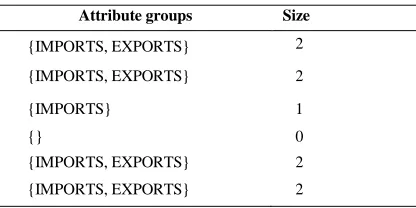
161 Table 1: Attribute Groups And Their Sizes
Attribute groups Size
{IMPORTS, EXPORTS} 2
{IMPORTS, EXPORTS} 2
{IMPORTS} 1
{} 0
{IMPORTS, EXPORTS} 2
{IMPORTS, EXPORTS} 2
Then, we will calculate the ratio of the space oc-cupied by the matching groups in the classes of C to the space needed to store the group A for the super-class S. Then, we compare it with a fusion threshold to decide whether to proceeds to merger or not.
In our example, this ratio is equal to 0.75. Indeed, the space occupied by all groups is 2 +2 +1 +0 +2 +2 = 9 units. While the space that will be occupied after the merger is 6 * 2 = 12 units. The report is equal to 9/12 = 0.75. Assuming that the merging threshold is 0.7, then we should proceed to merger in the group {IMPORTS, EXPORTS} of the super-class
COUNTRY.
After the merger, we remove the attributes EX-PORTS and IMPORTS from all classes Ci and we start again the same process of another group of attrib-utes until we obtain all data classes. In the next section, we will present our approach.
3. OUR APPROACH
Based on user interactions with the system, par-ticularly the distribution of their queries, we try in our approach to select the information more request-ed. The obtained data are classified for create the set of views candidates for materialization. Among the latter, we select those that will be effectively materialized.
3.1. Creating Candidate Views For Materializa-tion
In our approach, we assumed that a data pattern is present in user queries. i.e. some categories of data will be queried more frequently than other. Thus, it will be very useful to extract these patterns given the basis of which we will create the candidate views for materialization.
To do this, we will retrieve the attributes of inter-est. The latter are, then, classified as view schemas. Thereafter, we extract the most frequent constraints for each attribute and creating views. Now, we de-scribe each step in more detail.
3.1.1.Extracting attributes of interest.
Generally, in a mediation system, a global sche-ma representing the dosche-main of use is provided. It is in the terms of the latter are expressed the user que-ries. We analyze these queries in order to determine, among all the attributes of this schema, those in which users are interested.
Based on a set SQ=�Q1,Q2, …QNQ�of queries
posed previously, we calculate for each attribute Ai its frequency of appearance 𝑓𝐴
𝑖expressed by:
𝑓𝐴𝑖=
NA𝑖
NQ
Where NAi is the number of appearance of the at-tribute Ai and NQ the number of queries.
An attribute is considered as an attribute of inter-est if its frequency is higher than a threshold known as ATTRIBUTE-FREQUENCY. For this, we have de-fined the procedure EXTRACT-ATTRIBUTES.
SA={}; /*set of attribute of interest*/
EXTRACT-ATTRIBUTES(SQ) begin
SA0=get_All_Attributes(SQ);
NA0=cardinality(SA0) ; for i=1 TO NA0 then
NAi =0 ;
for ALL Q IN SQ then
S=get_All_Attributes(Q) ; if Ai IN S then
NAi = NAi+1; end if
end for
𝑓𝐴𝑖=NAi/NA0;
end for
for i=1 TO NA0 then
if 𝑓𝐴𝑖>INTEREST-FREQUENCY then
SA = SA UNION {Ai} end if
end for end
We then obtain the set SA={ A1, A2,…, AN} of at-tributes that will appear in the candidate views. It should be collected in compact classes, or what we called the “views schemas”. Thus, is that we present in the next section.
3.1.2.Creating view schemas
162 Different classification algorithms have been proposed. The most popular is k-means [24]. It partitions a dataset or points in k classes. Each class is represented by a center of gravity or centroid. From these centers, k-means calculates the distanc-es to various points and they are attributed to the nearest centroid.
Consider for example a dataset x1, x2,..., xN to classified into k disjoint classes Ci where 𝑖 ∈[1,𝑘], each one contains Ni points where 𝑁𝑖∈]0,𝑁[.
The basic idea is to share the points between dif-ferent classes while minimizing the intra-class dis-tance expressed by:
𝜏=� � ‖𝑥𝑡− 𝑐𝑖‖2
𝑥𝑡∈𝐶𝑖 𝑘
𝑖=1
where:
xt is a vector representing the tth point of the class
Ci, and ci it's centroid.‖xt−ci‖2is the geometric distance between the point xt and the center of the class Ci.
Thus, k-means is in three steps:
(i) Initialize randomly k center c1, c2, …, ck by data points.
For each point xt, and all k classes, repeating steps (ii) and (iii) until the sum of intra-classes distances cannot decrease.
(ii) Calculate the distance from xt to different cluster centers and assign it to that who’s centroid is the nearest.
(iii) Recalculate the centroids of the different classes.
In our case, it is impossible to define the cen-troids, and so we will not have the ability to calcu-late the distances.
To remedy this, we have associated to each pair of attributes, a value that represents the degree of dependency. The latter will be used to calculate the degree of dependency of an attribute to a class, also to calculate the degree of intra-class dependency. These values will be used, thereafter, to implement an algorithm, which we named k-schema to classi-fying attributes in classes or views schemas. 3.1.2.1.Degree of attribute-attribute dependency
This value is calculated by using the principle of voting. In other words, we votes 'one' for each pair of attributes appeared in the same query. We obtain, then, for each pair (A, B) ∈ SA × SA, a degree of dependency expressed by the following function:
𝜑 ∶ 𝑆𝐴𝑋𝑆𝐴 → ℕ
(𝐴,𝐵)→ �𝜑(𝐴,𝐵) 𝑖𝑓 𝐴 ≠ 𝐵
0 𝑖𝑓𝐴=𝐵
This function will be useful, then, to define the degree of dependency of an attribute to a class. 3.1.2.2.Degree of attribute-class dependency
Let 𝐶= {𝐴1,𝐴2, … ,𝐴𝑁 } a class and A an
attrib-ute.
The degree of dependency of attribute A to the class C is expressed by:
µ(𝐴,𝐶) =𝑁1� 𝜑(𝐴,𝐴𝑖) 𝑁
𝑖=1
We now have to define the graph of dependency between attributes of the same class.
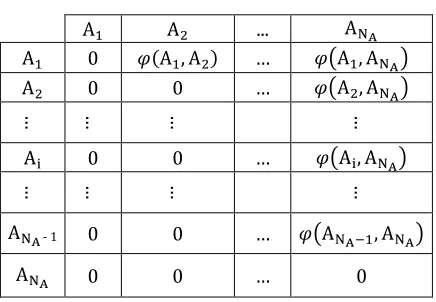
3.1.2.3.Matrix of attribute-attribute dependency From the set of attributes selected in the first step, we constructed the square matrix M = (mij) in NA size, defined by:
[image:5.612.313.531.433.584.2]𝑚𝑖𝑗 =�𝜑�𝐴0 𝑖,𝐴𝑗� 𝑖𝑓𝑖𝑓 𝑖 ≥ 𝑗𝑖<𝑗
TABLE I. MATRIX OF ATTRIBUTE-ATTRIBUTE DEPENDENCY
A1 A2 ... ANA
A1 0 𝜑(A1, A2) … 𝜑�A1, ANA�
A2 0 0 … 𝜑�A2, ANA�
… … … …
Ai 0 0 … 𝜑�Ai, ANA�
… … … …
ANAR- 1 0 0 … 𝜑�AN
A−1, ANA�
ANA 0 0 … 0
3.1.2.4.Degree of intra-class dependency
The degree of intra-class dependency is the sum of degrees of attributes dependencies in pairs. Thus for a class𝐶=�𝐴1,𝐴2, … ,𝐴𝑁𝐴�, the Degree of intra-class dependency is expressed by:
𝛿(𝐶) =𝑁𝐴(𝑁2
𝐴−1)� � 𝜑(𝐴𝑖,𝐴𝑗)
𝑁𝐴
𝑗=𝑖+1 𝑁𝐴
163 In the next section, we will present our algorithm. The latter is used to gather the classes of attributes that are most compact.
3.1.2.5.K- schema
K-schemas is an iterative algorithm to divide the attributes into k classes (schemas), while maximiz-ing the sum of intra-class dependencies expressed by:
τ=� δ(Ci) K
i=1
In other words, the objective is to maximize the dependency between the attributes of the same view. This is justified by the fact that if the views are more dependent the queries become less expen-sive in space and time.
Consider an example of a global schema with five attributes A1, A2, A3, A4, A5, and a matrix of attribute-attribute dependency as follows:
TABLE II. MATRIX OF ATTRIBUTE-ATTRIBUTE DEPENDENCY
A1 A2 A3 A4 A5
A1 2 6 3 8
A2 3 5 7
A3 2 1
A4 6
A5
We notice that the dependency between the at-tributes A1 and A5 is very high. This means that the chance that they appear in the same query is very high. Thus, our solution recommends to assign them to the same view.
Let us suppose that this recommendation has not been taken into account and these two attributes have been assigned to two different schemesV1(A3,
A5) and V2( A1, A2). In this case, it becomes neces-sary for satisfying queries that require the both attributes A1 and A5, and they are indeed many, to access to both views V1 and V2.
This query will contain a joint, thereby increas-ing its cost, which will be less high as if A1 and A5 were assigned to the same view.
K-schema has three steps:
(i) Define the number k of classes and initialize each one by an attribute such that they are
less dependent upon each other, in order to optimize the algorithm.
(ii) For each attribute, calculate its degree of de-pendency to different classes and assign it to the class to which is more dependent. (iii) Stop if the sum of degree of intra-class
de-pendencies τ cannot increase, otherwise re-turn to step (ii).
The result obtained in this step is a set of com-pact view schemas, subject we chose the right value of k number of views. Our solution is to calculate the value of k from the average number of attributes appeared in user queries. Thus, it is obtained by the following formula:
𝑘=𝜔N
Where:
N: the number of attributes of interest. 𝜔: the average number of attributes per query. In the next section, we should define for each schema, the values that will be taken by its attrib-utes.
3.1.3.Assigning constraints to attributes
Until now, we have defined the attributes most queried. We have gathered these attributes in com-pact classes. We should then define the attribute values (or constraints) for each view schema.
This phase is divided into three steps: (i) Extracting values of interest.
(ii) Definition of the most compact instances by assigning the values selected in the previous step to different attributes of each class. (iii) Merging instances of each class in a single. 3.1.3.1. Extracting values of interest
The extraction of values is to define for each at-tribute A, the set VA={ vi/ 1 ≤ i ≤ NVA} of values taken by this attribute. However, sometimes an attribute appears in a query without value. In this case, we add value ALL to the set of values taken by this attribute. This is justified by the fact that the user is interested in all values of this attribute.
Consider for example the following query: SELECT A
FROM S
164 SELECT A
FROM S
WHERE A = val
The attribute A has appeared with the value ‘val’ and also without value. In this case, the user is not interested in all values of attribute A, but only by the value 'val'.
In the example above, the query contains a con-straint expressed by the operator ‘=’. However, there may be other operators than ‘=’. These opera-tors depend on the type of the attribute A. We will subsequently define a procedure EXTRACT-VALUES
that receives the predicate specifying constraints as input and returns, as output, the set of values of interest, according to the operator and the type of the attribute:
The predicates specifying constraints are in gen-eral as ‘A operator V’ or ‘A operator B’, where A and
B are the attributes, and where V can be, according to the operator, either a value or a set of values.
In this paper we will limited to treating the first case ('A operator V') while postponing the second to future works.
EXTRACT-VALUES (Predicate)
begin
switch Type of A begin case ‘Boolean’:
switch operator begin case ‘=’
VA= VA∪{v}
case‘≠’ VA= VA∪{V�}
/*𝑉� is the complement of V*/ end switch
end case case ‘Text:
switch operator begin case ‘=’:
VA=VA∪{V}
case ‘≠’:
VA=VA∪{Vali/Vali≠V}
case ‘LIKE’:
VA=VA∪{Vali/Vali LIKE V}
case ‘NOT LIKE’:
VA=VA∪{Vali/Vali NOT LIKE V}
end switch end case
case ‘Numeric’:{ switch operator begin
case ‘=’: VA=VA∪{V}
case ‘≠’:
VA=VA∪{Vali/Vali≠V}
case ‘≥’:
VA=VA∪[V, MAX(Vali)]
case ‘≤’:
VA=VA∪[MIN(Vali),V]
case ‘>’:
VA=VA∪]V, MAX(Vali)]
case ‘<’:
VA=VA∪[MIN(Vali),V[
/*In the two following cases V is a set of values*/
case ‘IN’: VA=VA∪V
case ‘NOT IN’: VA=VA∪ V�
end switch end case end switch end
We have extracted for each attribute A, the set of values VA that he took. However, it is useless to
keep them all. We will eliminate those with the frequency less than a threshold known as VALUE
-FREQUENCY.
3.1.3.2. Definition of instances of classes
After selecting all values of attributes, we define, of each class, all instances possible by assigning values to their attributes. However, these instances should not appear in the final views. For selecting those that we will keep, we associate a degree of dependency on each pair of values taken by the pair of attributes (A, B).
3.1.3.2.1. Degree of attribute-attribute-values dependency
The degree of attribute-attribute-values depend-ency is calculated for each pair of values taken by a couple of attributes (A, B). Thus, is obtained for each pair of values (Vi, Vj)∈ VA × VB, a degree of dependency expressed by the following function:
𝜗A,B: VA× VB → ℕ
(Vi,Vj) → ϑA,B (Vi, Vj)
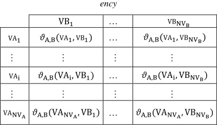
165 3.1.3.2.2. Matrix of attribute-attribute-values
dependency
From a sets SVA and SVB of values of the attrib-utes A and B, we constructed a matrix T=(tij) “
TA-BLE III.” in NVA× NVB size, where rows represent the values taken by attribute A and columns the values taken by the attribute B, and where:
[image:8.612.92.304.215.337.2]tij= 𝜗A,B (VAi,VBj).
Table III: Matrix Of Attribute-Attribute-Values Depend-ency
VB1 … VBNVB
VA1 𝜗A,B(VA1,VB1) … 𝜗A,B(VA1,VBNVB)
… … … …
VAi 𝜗A,B(VAi, VB1) … 𝜗A,B(VAi, VBNVB)
… … … …
VANVA 𝜗A,B(VANVA, VB1) … 𝜗A,B(VANVA, VBNVB)
3.1.3.2.3. Degree of intra-instance dependency The degree of intra-instance dependency is the sum of degrees of dependency per pairs of values. Thus, for instance I = {A1=V1,A2=V2, … ,AN=
VN}, the intra-instance dependency is expressed by:
δ(I) =NV1
ANVB� �𝜗A,B�VAi,VBj�
NVB
j=1 NVA
i=1
3.1.3.2.4. Definition of instances
It only remains now to define the instances of each class by assigning values to attributes. Then, we will keep, only, those in the degree of intra-instance dependency is higher than a threshold known as INSTANCE-DEPENDENCY.
Similarly, to the definition of view schemas, the objective at this stage also is to maximize the intra-instance dependencies. This is justified by the fact that if intra-instance dependencies are high, the data loads will occupy less storage space and at the same time satisfy more queries.
Consider the same matrix of attribute-attribute dependency ‘TABLE V.”, and Assuming that the attributes A1 and A5 often appear, respectively, with the values val1 and val5.
We have, in the case where A1 and A5 do not be-long to the same view, to load all data such as
A3=val3 and A5=val5for V1, and all data such as
A1=val1 and A2=val2 for V2.
In this case, we will have data that is more re-quested and that will not be materialized or other that are rarely requested and that will be material-ized. However, if we assigned A1 and A5 to the same view, in this case we will have to materialize, exactly the data that are requested by the majority of users. i.e. data such as A1=val1 et A5=val5. 3.1.4.Merging instances of each class
Until here, we have defined for each class, all in-stances. We selected those most queried. We will merge all instances of the same class in a single. We obtain thus, a candidate views for materializa-tion. The latter cannot be materialized all. Indeed, the space for materialization, the frequency of up-date and the cost of access to sources is critical. A set of selection criteria have been defined in [21] and [22], namely:
(i) The frequency of change: the views that rarely change are good candidates for materialization. (ii) The size of views: the views of small sizes are
favored for materialization than large ones. (iii) The availability of sources: The views, whose
data resides in sources that are rarely available, should be materialized.
(iv) The cost of access: the materialization of views whose data resides in sources with a high cost of access will improve the system perfor-mance.
Thus, a view will be materialized, if it satisfies at least two criteria.
4. EXPERIMENTATION AND EVALUATION
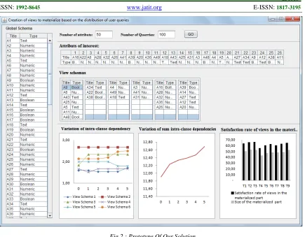
166 4.1. Experimentation
We have generated randomly a global schema. It is made up of 50 attributes A1, A2, …, A50. Then we generated also a random 100 queries Q1, Q2, … Q100 on this schema and wherein the threshold ATTRIB-UTE-FREQUENCY is equal to the average of the fre-quencies of attributes.
Our system has selected, based on the queries posed, the attributes of interest.(i.e. attributes highly requested). “Fig. 3”
Then, the algorithm k-schema was called. The latter has formed k classes of attributes or view schemas, where k is calculated by the formula 𝑘=N𝜔 presented above.
These schemas are then powered by assigning attributes to which they are more dependent. Thus, we have obtained the structure of the views pre-sented in “Fig.4”.
[image:9.612.96.531.71.410.2]Starting from this initial state, k-schema ex-change the attributes between schemas, while max-imizing the sum of the intra-class dependencies “Fig.5”.
Fig. 3: Attributs Of Interests
Fig. 4: Initial state of viewschemas
1st iteration :
2nd iteration :
[image:9.612.317.531.551.682.2]167 During the progress of the algorithm, the intra-classe dependencies vary depending on the immi-gration of attributes between schemas. Thus, we have represented that variation below “Fig.6”.
In this graph, the intra-class dependencies of cer-tain views increase while decreasing for others. However, we see in the graph below “Fig.7” That, despite the decrease in intra-class dependencies of certain patterns, the sum of these dependencies increases. This is justified by the fact that if an attribute migrates from one schema to another, it is because it is very dependent on the second than the first, which increases the final sum.
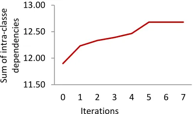
We then reiterate the algorithm a seventh and eighth once. We observed that the sum of the intra-class dependencies becomes constant. “Fig.8”
We repeated this operation with different exam-ples of global schema and different queries. Each time, we observe that the algorithm converges to a maximum value of the sum of the intra-class de-pendencies.
Until now, we have formed the view schemas. In the next section, we will assign values to the attrib-utes of each schema. To do this, our system has selected, based on queries posed on the system, a set of values for each attribute. For reasons of sim-plification, we will be limited to a single schema, and the same principle will be applied to the other. For example, consider the following schema: “Fig.9”
From the queries posed, the system has extracted for each attribute the set of values with which he appears through EXTRACT-VALUES function defined
1.00 1.50 2.00 2.50 3.00
0 1 2 3 4 5
Su
m o
f i
nt
ra
-c
la
ss
e d
ep
en
ci
es
Iterations
View Schema 1 View Schema 2
View Schema 3 View Schema 4
View Schema 5 View Schema 6
11.50 12.00 12.50 13.00
0 1 2 3 4 5 6 7
Su
m o
f i
nt
ra
-c
la
sse
de
pe
nde
nc
ie
s
Iterations 11.40
11.60 11.80 12.00 12.20 12.40 12.60 12.80
0 1 2 3 4 5
Su
m o
f i
nt
ra
-c
la
sse
de
pe
nde
nc
ie
s
[image:10.612.94.520.69.318.2]iterations
Fig. 8: Convergence Of K-Schema
3rd iteration :
4th iteration :
Fig. 5: Evolution Of The Structure Of View Schemas
Fig. 7: Variation Of The Sum Of Intra-Classe Dependencies
[image:10.612.321.519.308.425.2]5th iteration :
[image:10.612.96.290.395.557.2] [image:10.612.388.456.625.668.2]168 above, and for each two attributes, he extracted the degree of dependency in which they have appeared with two different values.
For reasons of simplification, we will not take all the values taken by the attributes. Thus, we ob-tained, for each pair of attributes, the matrices of attribute-attribute-value dependency presented below “Fig.10”.
Subsequently, the system will generate all in-stances of the schema in question by calculating the intra-instance dependencies. Then it will keep only those whose intra-instance dependence is greater than INSTANCE-DEPENDENCY,which is equal, in this case, to the average of intra-instance dependencies.
The following figure shows the intra-instance dependencies of each generated instances, and the threshold INSTANCE-DEPENDENCY that we took in this case equal to the average intra-instance de-pendencies.
According to the table in “Fig.12”, we keep I1, I2,
I3, I4, I5, I6, I8, I9. However, these last are included in I6. Then it will be itself a final candidate view for materialization.
By applying the same process for the other schemas, we will obtain all candidate views for materialization. Subsequently, we apply the
selec-tion criteria for choosing among them those that will be materialized.
4.2. Evaluation of the performance
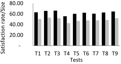
In this section, we will compare the rate of que-ries satisfied in the materialized part on the one hand, with the size of the materialized part relative to the size of data processed by the system on the other hand. To do this, we called our algorithm on several occasions and we calculated in each case the rate of satisfaction of queries in the materialized part. We calculated also the memory space occu-pied by the latter part compared to total memory space occupied by the data processed by the system. We obtained the graph shown in “Fig.13”.
In this graph, the black bars represent the rate of the queries satisfied in the materialized part, rela-tive to those satisfied virtually. As to the gray bars, they represent the rate of the space occupied by the materialized part relative to the total space occupied by the data processed by the system. For example, in test T3, the materialized data occupy 52.13%, whereas it satisfies 66.33% of queries.
We note that the rate of the space occupied by the materialized part is always less than the rate of queries satisfied in this part.
5. CONCLUSION AND OUTLOOKS
Selecting data to materialize in a hybrid mediator is a task crucial to the performance of the latter. Thus, a system of which the materialized part is well chosen is a system that consumes less memory space and in same time satisfies more queries. This will significantly reduce the response time of que-ries. Indeed, the response time of a query satisfied in whole or in part in the materialized part is always less than that satisfied virtually.
However, the materialized data is organized as views. Based on the distribution of user queries, we
20.00 40.00 60.00 80.00
T1 T2 T3 T4 T5 T6 T7 T8 T9
Sa
tis
fa
ct
io
n r
at
e/
Si
ze
Tests
Satisfaction rate of views in the materialized part Size of the materialized part
[image:11.612.321.520.288.393.2]Fig. 13: Satisfaction Rate Of Views In The Materialized Part
Fig. 10: Matrices Of Attribut-Attribut-Value Dependencies
[image:11.612.95.303.354.515.2]Fig. 12: Intra-Instance Depencies Fig. 11: Instances
I1 I2 I3 I4
I5 I6 I7 I8
169 proposed in this paper an approach to create these views.
In the first step, we extract the attributes most re-quested by users. These are classified as view schemas. To do this, we proposed an algorithm that we called k-schema. This iterative algorithm tries to maximize the sum of the intra-class dependencies.
We then extracted for each attribute, the most frequent values. The latter are assigned to the vari-ous attributes of each schema forming instances. We kept only those whose degree of intra-instance dependence is more than a threshold.
In our approach, we based only on the distribu-tion of user queries for the selecdistribu-tion of attributes that will appear in the views. It will be useful to exploit the user profile to obtain information about its interests and thus consider it in this phase.
We are based, also, on the appearance of attrib-utes in queries to calculate the degree of dependen-cy. It is possible to exploit the domain ontology to calculate this dependency.
In our approach, the selection of data to material-ize is a task done at the time of the establishment of the system. This makes static our solution. In other words, there will be no evolution of the material-ized part. However, the choices and the interests of users may change over time. It is very important to add a dynamic aspect, taking into account the changes that may appear in the choices and the interests of users.
REFRENCES:
[1] Haas, L. M. Beauty and the beast: The theory and practice of information integration. In ICDT, pages 27_43. (2008).
[2] A. Elmagarmidet al. Management of Hetero-geneous and Autonomous Database Systems. Morgan Kaufmann, San Francisco, 1999. [3] A. Zellou. Contribution à la réécriture LAV
dans le contexte de WASSIT, vers un Frame-work d’intégration de ressources. Thèse de Doc-torat. Rabat. Maroc. Avril 2008.
[4] Y. Arens, C. Y. Chee, C.-N. Hsu and C. A. Knoblock. Retrieving and Integrating Data from Multiple Information Sources," in Intl Journal of Intelligent and Cooperative Informations Systems. June 1993.
[5] S. Chawathe, H. Garcia-Molina, J. Hammer, K. Ireland, Y. Papakonstantinou, J. Ullman, and J. Widom. The TSIMMIS pro ject: integration of heterogeneous information sources. IPSJ Conference, Tokyo, 1994.
[6] V.S. Subrahmanian, S. Adali, A. Brink, R. Emery, J. Lu, A. Ra jput, T. Rogers, R. Ross, and C. Ward. HERMES: A heterogeneous rea-soning and mediator system. Technical report, University of Maryland, 1995.
[7] T. Kirk, A. Y. Levy, Y. Sagiv, D. Srivastava . The Information Manifold. In proceedings of the AAAI-95 Spring Symposium on Infor-mation Gathering from Heterogeneous, Distrib-uted Environments.1995
[8] A. Y. Levy, A. Rajaraman and J. Ordille (1996). Query answering algorithms for infor-mation agents. In proceedings of the 13the Na-tional Conference on Artificial Intelligence (AAAI-96). 1996.
[9] V. Lattes and M. Rousset. The use of CARIN language and algorithms for Information Inte-gration: the PICSEL project. proceedings of the 2nd international and workshop on intelligent information integration, Brighton Centre, Brighton, interdisciplinary UK, August 1998. [10] V. Aguilera, S. Cluet, P. Veltri, D. Vodislav
and F. Wattez. Querying XML Documents in Xyleme. in Proceedings of the ACM SIGIR 2000 Workshop on XML and Information Re-trieval. 2000.
[11] J. Widom. « Integrating Heterogeneous Da-tabases: Lazy or Eager? », ACM Computing Surveys 28A(4), Décembre 1996
[12] R. Hull, G. Zhou, University of Colorado. « A Framework for Supporting Data Integration Using the Materialized and Virtual Approach-es”. SIGMOD ’96 6/96 Montreal, Canada.1996. [13] J. McHugh, et al., Stanford University.Lore:
A Database Management System for Semistruc-tured Data. 1997.
[14] N. Ashish, C. A. Knoblock and C. Shahabi, “selectively materializing data in mediators by analyzing user queries”, in Fourth IFCIS Con-ference on Cooperative Information Systems, pages, 1999.
[15] N. Ashish, “optimizing information media-tors by selectively meterializing data”,Ph.D dis-sertation, Departement of computer Science. faculty of the graduate school, university of southern california, 2000.
170 [17] Y. Papakonstantinou,V. Vassalos .
Architec-ture and Implementation of an XQuery-based Information Integration Platform. Bulletin of the Technical Committee on Data Engineering March 2002 Vol. 25 No. 1.pages 18-26. 2002. [18] S. Kermanshahani : “IXIA (IndeX-based
Integration Approach) A Hybrid Approach to Data Integration”, Thèse, Université Joseph Fourier – Grenoble I, 2009.
[19] W. Hadi., A. Zellou, B. Bounabat, “Toward classification of hybrid integration systems”, in 22nd edition of ICSSEA, Paris, France, 2010. [20] S. Anter, A. Zellou, W. Hadi, “the hybrid
integration systems: A comparative study”, in 1th edition of JDSIRT, Rabat, Maroc, 2012. [21] V. Y. Bichutskiy, R. Colman, R. K..
Barchmann and R. H. Lathrop, “Heterogeneous Biomedical Database Integration Using a Hy-brid Strategy: A p53 Cancer Research Data-base”. Cancer Informatics 2006.
[22] W. Hadi., A. Zellou and B. Bounabat, “Hy-brid information integration: fuzzy controller for selecting views to materialize”, in 7th edi-tion of SITA, Mohmmedia, Maroc, 2012. [23] G. Wiederhold. Mediators in the architecture
of future information systems, The IEEE Com-puter Magazine, Mars 1992.