SECURE ROUTING IN MANET USING ASYMMETRIC GRAPHS

FLOW PATTERN IDENTIFICAITON OF OIL-GAS-WATER

THREE-PHASE FLOW BASED ON NPSO-LSSVM

ALGORITHM

1_{YINGWEI LI,} 2_{RONGHUA XIE,} 1_{LINA YU}

1

College of Information Science and Engineering, Yanshan University, Qinhuangdao 066004, Hebei,China

2 _{Logging & Testing Services Company, Daqing Oilfield Co.LTD, Daqing 163100, Heilongjiang, China}

ABSTRACT

In this paper, a hybrid particle swarm optimization based on the natural selection (NPSO) was presented and used to optimize the parameters of Least Square Support Vector Machine (LSSVM). The NPSO algorithm overcomes the shortcomings of premature convergence and poor local search capability of traditional Particle Swarm Optimization (PSO). Then a classification model of oil-gas-water three-phase flow patterns was established based on NPSO-LSSVM to identify three typical water-based flow patterns of oil-gas-water three-phase flow including bubbly flow, slug flow and bubbly-slug flow. By combining the statistics analysis, Hilbert-Huang transformation, complexity measure analysis, chaotic recurrence quantification analysis and chaotic fractal analysis, the conductance fluctuation signal of oil-gas-water three-phase flow in the vertical pipe was analyzed. The nine feature parameters reflecting the changes of oil-gas-water three-phase flow were extracted and used as the input vectors of the NPSO-LSSVM classification model. Simulation results showed that the correct identification rate of the oil-gas-water three-phase flow patterns was 94%, and it indicated that the classification model proposed in this paper was reasonable and had a practical value.

Keywords: LSSVM, NPSO, Feature Extraction, Flow Pattern Identification

1. INTRODUCTION

Oil-gas-water three-phase flow widely exists in the oil exploration, nuclear reactors and other chemical industry fields. The accurate identification of oil-gas-water three-phase flow patterns is of great significance. However, three-phase flow is a complex nonlinear system which exists interface effect and relative velocity. So the accurate identification of oil-gas-water three-phase flow patterns is still a quite difficult work. Since the 1990s, a variety of intelligent calculation methods have been applied to flow pattern identification of multiphase flow. Trafalis et al. identified the transition region between gas-liquid two-phase flow patterns in vertical and horizontal pipes using multi-class Support Vector Machine (SVM) [1]. By using SVM classifier, Zhang et al. identified four kinds of flow patterns of oil-gas two-phase flow, including stratified flow, annular flow, core flow and full-pipe flow [2].

SVM is a pattern recognition method based on the principle of structural risk minimization. It can effectively solve the problems with small sample, high dimension and local minimal point. However,

it has the shortcomings of a slow computing speed and a poor robustness. LSSVM is an extension of standard SVM, and it uses least squares linear systems as the loss function instead of the quadratic programming method used by standard SVM, therefore the computation is simplified. The core of LSSVM is the precise parameter setting of the regularization and the kernel function. In recent years, many algorithms have been proposed to optimize these parameters, such as the Particle Swarm Optimization (PSO) algorithm, Genetic Algorithm (GA) and Ant Colony Optimization (ACO) algorithm. Compared with the GA algorithm and the ACO algorithm, the PSO algorithm has the advantages of less memory usage, fast convergence speed and fewer adjustable parameters [3]. However, there are a number of drawbacks in the evolutionary process of PSO algorithm, such as premature convergence and poor local search capability [4].

oil-gas-water three-phase flow namely mean, skewness, the second and the eighth kurtosis coefficients of intrinsic mode function, entropy, power spectral entropy, approximate entropy, Hurst exponent and correlation dimension were used as the input vectors of the model. Three kinds of typical water-based flow patterns of oil-gas-water three-phase flow, including bubbly flow, slug flow and bubbly-slug flow, were identified effectively with this classification model.

2. NPSO-LSSVM ALGORITHM

Classification problems of LSSVM model can be described as the following equation [5].

2 2

1

min . ( , ) 2 , 0

2

. . [ ( ) ] 1 , 1, 2, ,

N i i T

i i i

J

s t y x b i N

γ

ω ξ ω ξ γ

ω φ ξ

=



= + ∑ >

 

 _{+ = − =}

 L

(1)

Where J( , )ω ξ represents risk of the structure;

ωmeans the weight vector;

γ

is the regularization factor; 2

i

ξ is the loss function;

φ

( )

x

_i denotes the mapping function of nuclear space. The Lagrange function is defined as follows:

1

( , , , ) N { T ( ) 1 }

i i i i

i

Lω ξ αb J α y ω φ x b ξ

=

= −∑ + − + (2)

Where α_i is the Lagrange multiplier. Compute derivatives for the formula (2) and define the optimal conditions: ∂ ∂ =L ω 0 , ∂ ∂ =L b 0 ,

0

L ξ

∂ ∂ = , ∂ ∂ =L α_i 0 . Then LSSVM classification function is obtained by solving these linear equations:

1

( )

sgn(

n i i

( , )

i

)

i

y x

α

y k x x

b

=

∑

=

+

(3)

In this paper, RBF kernel function is used as the mapping function of nuclear space. In LSSVM modeling, a larger regularization parameter γ will lead to a poor promotion ability. And a larger nuclear function parameter σ2 _{will increase the}

experience risk. On the contrary, the anti-interference ability decreases and an over-fitting phenomenon is introduced easily. Therefore, it is necessary to globally optimize the parameters of LSSVM.

Traditional PSO algorithm begins with a random swarm of N particles. Each particle representing a point in the solution space has M unknown parameters to be optimized. In iteration, the particles update themselves by tracking their own optimal value (individual extreme value) and groups’ optimal value (global extreme value). And the merits and demerits of particles are evaluated by the fitness function. The dimension of the

complex space d is assumed. In the nth iteration, the ith particle is represented by a position vector

( )

i

x n

and a velocity vector

v n

_i

( )

. Thus, the positions set and the velocities set are defined:

( )

( )

( )

( )

( ) ( )

( )

1 1 2 2 , , , , , ,

( )

M

M

X n x n x n x n

V n v n v n v n

= =  _ _         L L (4)

Then the status of a particle is updated by the following equations.

1 1 2 2

( 1) ( ) [ ( ) ( )]

[ ( ) ( )]

( 1) ( ) ( 1)

i i i

i i

i i i

V n w V n c r Pbest n X n

c r Gbest n X n

X n X n V n

 _{+ = ⋅ + ⋅ ⋅ −}  + ⋅ ⋅ −   + = + +  (5)

Where

w

is the inertia weight factor;

c

₁ and

c

₂

are the acceleration coefficients;

r

₁ and

r

₂ are random variables between 0 and 1.

Although the PSO algorithm has a simple calculating process, easy implementation and fast convergence speed, it has many deficiencies. On one hand, its initialization is at random. On the other hand, it is very easy to reach a local optimal solution. Therefore, a hybrid particle swarm optimization based on the natural selection (Nature Selection and Breed PSO, NPSO) is presented in this paper, adopting ideas from the GA algorithm and natural selection mechanism. The regularization parameter

γ

and RBF kernel parameter σ2

of LSSVM are optimized by NPSO algorithm according to the following steps.

Step 1: Both training samples and test samples are composed by the extracted feature parameters, and then are normalized.

Step 2: Initialize Parameters of the population. The size of the population is 1000 and the number of iterations is 100. Use a linear decreasing weighting method with the formula:

(

)

0.9 0.9 0.1 100

w= − ∗t − .Where wmax and wmin

are 0.9 and 0.1 respectively. Both c and ₁ c are 2. ₂

The solution space is two-dimensional. The range of

γ

is from 1 to 5000, and the range of σ2 _{is from} 0.1 to 10000. The crossover probability P is 0.9. c

Step 3: Evaluate the fitness of each particle. The fitness function F is determined by the correct identification rate of LSSVM classification model.

Define the fitness function:

( )

1

n _{i i}

i _i

F

i

u

u

u

∗

=

−

=

∑

,

(i=1, 2,L, )n , where u and i ui

∗ _{are actual value}

and predicted value of sample

i

.

Step 4: For each particle, compare the fitness

( )

if F i

( )

>F pbest( ) ,

pbest

=

i

. Compare the

fitness F i of all particles with the global extreme

( )

valueF gbest , if

(

)

F i

( )

>F gbest

(

)

,

gbest

=

i

.

Step 5: Update the position and speed of the particle according to the formulas (5).

Step 6: Rank all particles in the population in order of the fitnessF i . Produce a random number

( )

between 0 and 1. If this number is smaller than the crossover probability, the best half of the particles is selected as parent particles. Then put them into a chiasmatic cistern and cross with each other according to the formula:

1 2

1 2

1

1 2

( ) ( ) (1 ) ( )

( ) ( )

( ) ( )

( ) ( )

c c

child x p parent x p parent x

parent v parent v

child v parent v

parent v parent v

= ⋅ + − ⋅ 



+ 

= ⋅

 ₊



(6)

Step 7: Replace the poor half of the particles with the same number of child particles. And their location and speed are restricted.

Step 8: If this process satisfies a stopping condition, go to step 9. Otherwise, go to step 3.

Step 9: Output the global optimal solution. As a population is divided into several subgroups in NPSO algorithm, the crossover operation can be executed not only in the same subgroup, but also in different ones. It not only has faster convergence, higher searching precision, but also avoids the shortcomings of time-consuming and blind of the grid search method.

3. DATA PROCEDDING AND ANALYSIS

The experiments were carried out on a three-phase flow simulation test device. The device consists of a transparent plexiglass test pipe with 8 meters in length and 125 millimeters’ inner diameter, an oil-water separating tank, a buffer tank, two overhead tanks, several control systems and other components. Besides that, the experiments used a conductance correlation flow meter with 20 millimeters’ inner diameter in the test section. It is made up of a fan current collector, a six-electrode conductivity sensor and a drive circuit system, etc. The schematic diagram of oil-gas-water flow loop is shown in Figure 1. In the experiments, the experimental fluids were diesel oil, air and water. Air was supplied from an air compressor, and flows through a gas cleaning equipment into a gas buffer tank. Oil and water were supplied from an oil tank and a water tank, and flowed into an oil overhead tank and a water overhead tank through oil pump and water pump, respectively. Then air, oil and water from the buffer

[image:3.612.314.522.194.285.2]

tank or the overhead tanks flowed into the plexiglass test pipe after being measured by the turbine flow meter, and they streamed from bottom to top. Air from the test pipe was discharged directly. The water mixture was put into the oil-water separating tank. After gravity separation, oil and water flowed into the oil tank and the water tank respectively for cycling utilization.

Figure 1: The Schematic Of Oil-Gas-Water Flow Loop

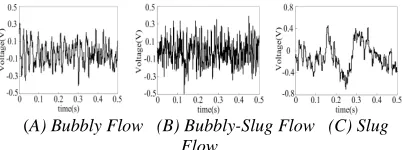
Because China's onshore oil field generally had a high moisture content and a low-yielding liquid, in the experiments, the total flow rate of oil-gas-water three-phase flow varied from the range of 5m3/d to 80m3/d. Moisture content varied from the range of 50% to 90%. Oil content varied from the range of 5% to 30%. Gas content varied from the range of 5% to 30%. The experimental program is shown as follows: first, a fixed water-phase flow rate is put into the pipeline; Then increase the oil-phase flow rate and the gas-oil-phase flow rate in the pipeline gradually; After matching the oil phase, gas phase and water phase one time, observe the flow patterns of oil-gas-water three-phase flow by visual observation. In the experiments, three kinds of typical water-based flow changes are observed, and there are bubbly flow, bubbly-slug flow and slug-flow. In the experiments, 99 conductivity fluctuation signals of oil-gas-water three-phase flow were collected in all. The conductance fluctuation signals of the three kinds of typical water-based flow patterns are shown in Figure 2.

(A) Bubbly Flow (B) Bubbly-Slug Flow (C) Slug Flow

[image:3.612.318.519.574.649.2]

4. IDENTIFICATION INSTANCE OF OIL-GAS-WATER FLOW PATTERN

In this article, a LSSVM model based on NPSO optimization was adopted to identify the three kinds of typical water-based flow patterns of oil-gas-water three-phase flow. The classification model is shown in Fig. 3. In the layer of feature selection, nine feature parameters were extracted from the angle of complementary features to use as the input vectors of the model. Two statistical feature parameters, mean and skewness, were extracted in time domain based on the statistics analysis. Utilizing the Hilbert-Huang transformation and the complexity measure analysis, the second and the eighth kurtosis coefficients of intrinsic mode function, power spectral entropy and approximate entropy were selected in the time-frequency

domain. With the chaotic recurrence quantification analysis, a recursive quantification index, termed entropy, was extracted. Two fractal parameters, Hurst exponent and correlation dimension, were selected with the chaotic fractal analysis. The

extraction methods had seen the literature report [6]; In the layer of network optimization, the input vectors were normalized firstly. Then the regularization parameter γ and the RBF kernel

parameter σ2

[image:4.612.104.511.299.563.2]

of LSSVM were optimized with the NPSO algorithm; In the layer of flow pattern identification, the training sample set was used to train the network. After the training, the flow patterns which belonging to the actual test object were identified. Where the output results of bubbly flow, bubble-slug flow and slug flow would be ‘1’, ‘0’ and ‘-1’, respectively.

Figure 3: NPSO-LSSVM Classification Model

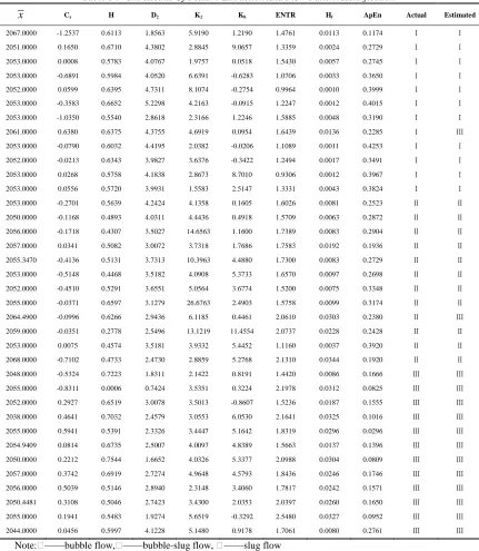
Select 63 samples from the 99 ones of conductance fluctuating signal of oil-gas-water three-phase flow and form the training sampled set, in which 21 samples for each one of the three kinds of typical flow patterns, bubbly flow, bubble-slug flow and slug flow respectively. Meanwhile, the test sampled set was made up of the remaining 36 samples, 12 samples for each flow pattern. The feature extraction and flow pattern identification results of the 36 test samples are shown in Table 1. It showed that NPSO-LSSVM classification model correctly identified 34 samples, and the overall identification

rate was 94%. And the correct identification rate of slug flow was 100%. Each one of bubbly flow and bubbly-slug flow misidentified one case, and their correct identification rate was both 92%.

generalization ability. If the number of training samples increases, the false identification can be reduced. However, the correct identification rate of 94% of the NPSO-LSSVM classification model is

[image:5.612.91.522.158.653.2]

sufficient to meet the needs of the actual projects. Therefore, the methods of feature extraction and flow pattern classification are reasonable and have a practical value.

Table 1 : The Results Of Feature Extraction And Flow Pattern Identification

x Cx H D2 K2 K8 ENTR Hf ApEn Actual Estimated

2067.0000 -1.2537 0.6113 1.8563 5.9190 1.2190 1.4761 0.0113 0.1174 Ⅰ Ⅰ

2051.0000 0.1650 0.6710 4.3802 2.8845 9.0657 1.3359 0.0024 0.2729 Ⅰ Ⅰ

2053.0000 0.0008 0.5783 4.0767 1.9757 0.0518 1.5430 0.0057 0.2745 Ⅰ Ⅰ

2053.0000 -0.6891 0.5984 4.0520 6.6391 -0.6283 1.0706 0.0033 0.3650 Ⅰ Ⅰ

2052.0000 0.0599 0.6395 4.7311 8.1074 -0.2754 0.9964 0.0010 0.3999 Ⅰ Ⅰ

2053.0000 -0.3583 0.6652 5.2298 4.2163 -0.0915 1.2247 0.0012 0.4015 Ⅰ Ⅰ

2053.0000 -1.0350 0.5540 2.8618 2.3166 1.2246 1.5885 0.0048 0.3190 Ⅰ Ⅰ

2061.0000 0.6380 0.6375 4.3755 4.6919 0.0954 1.6439 0.0136 0.2285 Ⅰ Ⅲ

2053.0000 -0.0790 0.6032 4.4195 2.0382 -0.0206 1.1089 0.0011 0.4253 Ⅰ Ⅰ

2052.0000 -0.0213 0.6343 3.9827 3.6376 -0.3422 1.2494 0.0017 0.3491 Ⅰ Ⅰ

2053.0000 0.0268 0.5758 4.1838 2.8673 8.7010 0.9306 0.0012 0.3967 Ⅰ Ⅰ

2053.0000 0.0556 0.5720 3.9931 1.5583 2.5147 1.3331 0.0043 0.3824 Ⅰ Ⅰ

2053.0000 -0.2701 0.5639 4.2424 4.1358 0.1605 1.6026 0.0081 0.2523 Ⅱ Ⅱ

2050.0000 -0.1168 0.4893 4.0311 4.4436 0.4918 1.5709 0.0063 0.2872 Ⅱ Ⅱ

2056.0000 -0.1718 0.4307 3.5027 14.6563 1.1600 1.7389 0.0083 0.2904 Ⅱ Ⅱ

2057.0000 0.0341 0.5082 3.0072 3.7318 1.7686 1.7583 0.0192 0.1936 Ⅱ Ⅱ

2055.3470 -0.4136 0.5131 3.7313 10.3963 4.4880 1.7300 0.0083 0.2729 Ⅱ Ⅱ

2053.0000 -0.5148 0.4468 3.5182 4.0908 5.3733 1.6570 0.0097 0.2698 Ⅱ Ⅱ

2052.0000 -0.4510 0.5291 3.6551 5.0564 3.6774 1.5200 0.0075 0.3348 Ⅱ Ⅱ

2055.0000 -0.0371 0.6597 3.1279 26.6763 2.4903 1.5758 0.0099 0.3174 Ⅱ Ⅱ

2064.4900 -0.0996 0.6266 2.9436 6.1185 0.4461 2.0610 0.0303 0.2380 Ⅱ Ⅲ

2059.0000 -0.0351 0.2778 2.5496 13.1219 11.4554 2.0737 0.0228 0.2428 Ⅱ Ⅱ

2053.0000 0.0075 0.4574 3.5181 3.9332 5.4452 1.1160 0.0037 0.3920 Ⅱ Ⅱ

2068.0000 -0.7102 0.4733 2.4730 2.8859 5.2768 2.1310 0.0344 0.1920 Ⅱ Ⅱ

2048.0000 -0.5324 0.7223 1.8311 2.1422 0.8191 1.4420 0.0086 0.1666 Ⅲ Ⅲ

2055.0000 -0.8311 0.0006 0.7424 3.5351 0.3224 2.1978 0.0312 0.0825 Ⅲ Ⅲ

2052.0000 0.2927 0.6519 3.0078 3.5013 -0.8607 1.5236 0.0187 0.1555 Ⅲ Ⅲ

2038.0000 0.4641 0.7032 2.4579 3.0553 6.0530 2.1641 0.0325 0.1016 Ⅲ Ⅲ

2055.0000 0.5941 0.5391 2.3326 3.4447 5.1642 1.8319 0.0296 0.0296 Ⅲ Ⅲ

2054.9409 0.0814 0.6735 2.5007 4.0097 4.8389 1.5663 0.0137 0.1396 Ⅲ Ⅲ

2050.0000 0.2212 0.7544 1.6652 4.0326 5.3377 2.0988 0.0304 0.0809 Ⅲ Ⅲ

2057.0000 0.3742 0.6919 2.7274 4.9648 4.5793 1.8436 0.0246 0.1746 Ⅲ Ⅲ

2056.0000 0.5039 0.5146 2.8940 2.3148 3.4060 1.7817 0.0242 0.1571 Ⅲ Ⅲ

2050.4481 0.3108 0.5046 2.7423 3.4300 2.0353 2.0397 0.0260 0.1650 Ⅲ Ⅲ

2055.0000 0.1941 0.5483 1.9274 5.6519 -0.3292 2.5480 0.0327 0.0952 Ⅲ Ⅲ

2044.0000 0.0456 0.5997 4.1228 5.1480 0.9178 1.7061 0.0080 0.2761 Ⅲ Ⅲ

5. CONCLUSIONS

(1) The NPSO algorithm is realized by introducing the GA algorithm and natural selection mechanism into the PSO algorithm. This algorithm overcomes the problems of premature convergence

and the tendency to fall into the local optimum in traditional PSO algorithm. On this basis, the NPSO algorithm is used to optimize the regularization parameter γ and RBF kernel parameter σ2

of the LSSVM model. The convergence speed and the recognition accuracy of the model are improved.

(2) A classification model of oil-gas-water three-phase flow patterns is established based on the NPSO-LSSVM algorithm to identify the three kinds of typical water-based flow patterns of oil-gas-water three-phase flow. Nine feature parameters including mean, skewness, the second and the eighth kurtosis coefficients of intrinsic mode function, entropy, power spectral entropy, approximate entropy, Hurst exponent and correlation dimension are extracted and used as its input vectors. The experiment results showed that the accurate identification rate of the three kinds of typical flow patterns was 94%, which distinguished well the differences of each flow pattern.

ACKNOWLEDGEMENTS

This work was supported by National S&T Major Project of China (No.2011ZX05020-006), National Science Foundation of China (No.61071200), Hebei Science Foundation of China(No.2010001297).

REFERENCES:

[1] Trafalis T., Oladunni O., Papavassiliou D, “Two-phase flow regime identification with a multiclassification support vector machine (SVM) model”, Industrial and Engineering

Chemistry Research, Vol. 44, No. 12, 2005,pp.

4414-4426.

[2] Zhang L. F., Wang H. X, “Identification of oil-gas two-phase flow pattern based on SVM and electrical capacitance tomography technique”,

Flow Measurement and Instrumentation, Vol.

21, No. 1, 2010,pp. 20-24.

[3] Taher S. A., Karimian A., Hasani M, “A new method for optimal location and sizing of capacitors in distorted distribution networks using PSO algorithm”, Simul Model Pract

Theory, Vol. 19, No. 2, 2011, pp. 662-672.

[4] Ziari I., Ledwich G., Ghosh A, “Optimal integrated planning of MV-LV distribution systems using DPSO”, Electric Power Systems

Research, Vol. 81, No. 10, 2011,pp. 1905-1914.

[5] Suykens J. A. K, Vandewalle J, “Least squares support vector machine classifiers”, Neural

Processing Letters, Vol. 9, No. 3, 1999,pp.

293-300.

[6] Li Y. W., Xie N., Kong L. F, “Chaotic recurrence analysis of oil-gas-water three-phase flow in vertical upward pipe”, Information

Technology Journal, Vol. 10, No. 12, 2011,pp.