TRAINING AND DEVELOPMENT OFARTIFICIAL NEURAL NETWORK MODELS: SINGLE LAYER FEEDFORWARD AND MULTI LAYER FEEDFORWARD NEURAL NETWORK

(1)

ISSN: 1992-8645 www.jatit.org E-ISSN: 1817-3195

TRAINING AND DEVELOPMENT OFARTIFICIAL NEURAL

NETWORK MODELS: SINGLE LAYER FEEDFORWARD

AND MULTI LAYER FEEDFORWARD

NEURAL NETWORK

1 _{VIDYULLATHA PELLAKURI,}2_{D. RAJESWARA RAO}

1

Research scholar, Department of CSE, KL University, Guntur, Andhra Pradesh

*2

Professor, Department of CSE, KL university, Guntur, Andhra Pradesh

E-mail: [email protected]

ABSTRACT

Research in the artificial neural network has been attracting and most successful technology in recent years. Though the first model of artificial neurons was presented by Warren McCulloch and Walter Pitts in 1943, the new models have been raised even in the recent years. Some of the problems are solved by mathematical analysis but it leaves many queries openly for further developments. Anyway, the study of neurons, their interconnected nodes and their actions as the brains primary building blocks is one of the most important research fields in modern biology. The purpose of this research paper is to provide how to learn the logic behind the architectures, methodologies of artificial neural networks. This study consists of two parts: the first part shows the learning of single layer feed forward neural network (SLFFNN) architecture where as in second part the multi layer feed forward (MLFFNN) back-propagation neural network covers the learning and training of optimization techniques.

Keywords: Artificial Neural Network, Back-Propagation Neural Network, Learning Rate, Momentum, Multi Layer Perceptron.

1. INTRODUCTION

An artificial neural network model has a similar structure of human brain which computes parallel processing of information. A neural network system consists of neurons which are interconnected and processing them is accompanied in fig 1. The network architecture is a set of inputs, computing units and output nodes. The input nodes are the just entry nodes for information in to the network but they do not perform any computation paradigm. The network architecture consists of set of computing units m is subdivided in to n subsets such that m1,m2,m3,….mn; in such a way that the

connections are associated from m1 to m2 and to m1 and the units of subset of mn are the only ones

connected to the target node. In this network, the input nodes is called input layer and the subsets of mn are called layers of the network, the set of

output nodes is called output layer where as remaining layers with no direct connections from or

towards the outside are called hidden layers. In layered network all nodes from one layer are connected to all other nodes to the following layer.

(2)

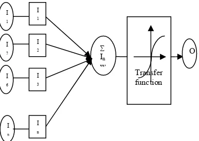
[image:2.612.97.291.394.532.2]

outcomes. In fact neural network have many interesting properties but to improve the performance ‘learning’ is the most important step. Learning methods are by two types such as supervised and unsupervised methods. In supervised learning method, some inputs are collected and presented to the network where the output is generated so that the error is measured from the actual value to the net generated value and the weights are updated according to the error calculated. This kind of learning is also called learning with the guidance of a teacher because a control process knows the exact output for the collected inputs. In unsupervised learning for the given input, the exact output is unknown for which a network generates. The supervised learning is further classified in to a method called reinforcement or error correction. Perceptron learning algorithm is a one of the example of supervised learning with reinforcement. The network topology depends upon the inputs and outputs, number of training samples, the strength of noise, activation function and complexity of the problem. The information flow for a neural network model is shown in figure1.

Figure 1: Neural Network Model: Information Flow From Left to Right

2. LITERATURE SURVEY

In July 2015, pellakuri etal [1] analyzes the comparative study on Multivariate Regression Analysis (MVRA) versus back propagation neural network model with structure 4-1-1 has been chosen as appropriate model according to three statistical indexes MAE, RMSE and R2 analysis, the performance parameters in artificial neural network using back propagation yields 99% accuracy for prediction. In same year, Vidyullatha pellakuri [9] gave an idea about environmental data Forecasting based on the data mining classification

techniques using WEKA and suggested that Regression model is the best practice method to predict output for Quality of ambient dataset with WEKA. In 2013, Fardis nakhaei etal [2] uses two techniques such as ANN and statistical methods to estimate Cu grade and recovery values in flotation column concentrate. According to him, BPNN is effective for predicting metallurgical performance of flotation column. Similarly he has also been observed that RBFNN (radial basis function neural network) based prediction systems achieve faster convergence compared to BPNN (back propagation neural network) based system but with higher levels of prediction errors and also, for performance improvement he considers additional program such as genetic algorithms (GA) and fuzzy systems. Anyaeche C. O etal (2013) [3] uses artificial neural network, Back Propagation Artificial Neural Network (BP-ANN), as an alternative predictive tool to multi-linear regression, for establishing the interrelationships among productivity, price recovery and profitability as performance measures and It was observed that BA-ANN model has Mean Square Error (MSE) of 0.02 while Multiple Linear Regression (MLR) has MSE of 0.036 which concludes that artificial neural network is a more efficient tool for modeling interrelationships among productivity, price recovery and profitability. IN 2012, Asghar Azizi etal [4] studied, two techniques such as back propagation neural network (BPNN)and multiple linear regression (MLR) were applied to estimate gold recovery in cyanide leaching process. The designed neural network has three layers including input layer (seven neurons), hidden layer (ten neurons) with tansig activation function and output layer (one neuron) with linear activation function. The comparison between the estimated recoveries and the measured data resulted in the correlation coefficients, R, 0.952 and 0.884 for training and test data using BPNN model. However, the R values were 0.786 and 0.767 for training and test data respectively, by MLR method. In addition, the root mean square (RMS) error obtained 1.08 and 1.22 for BPNN and MLR methods, respectively. In 2010, Maitha H etal [5] used MATLAB tools to predict monthly average global solar radiation by eleven models with different input combinations are modeled with MLP and RBF ANN techniques with performance of 90 % and low MBE, MAPE and RMSE values. Gang Sun etal proposes Back-propagation (BPNN) and generalized regression neural network (GRNN) methods on the measurements of diurnal and seasonal NH3, H2S, CO2, and PM10 levels and emissions from deep‐pit swine buildings and he

I 1

I 2

I 6

I n

I 1 w

I 2 w

I 3 w

I n w

∑

In

w

Transfer function

(3)

was found that the obtained results of BPNN and GRNN predictions were in good agreement with the actual measurements, with coefficient of determination (R2) values between 81.15% and 99.46%. Other significant characteristics of the GRNN in comparison to the BPNN were the excellent approximation ability, fast training time and exceptional stability during the prediction stage. So, he recommended that a generalized regression neural network (GRNN) be used instead of a back-propagation neural network in source air quality modeling. Grivas et al., 2006 Sousa et al.,2007 [6] show that ANN black‐box models are able to learn nonlinear relationships with limited knowledge about the process structure, and the neural networks generally present better results than traditional statistical methods. Jacek M. Zurada [8] discussed Very simple structure and easy to understand to start with ANN. This current work focuses the logic to learn a single feed forward and multiple feed forward neural network models and the results are shown by implementing neural network models in c programming language.

3. METHEDOLOY

3.1 Single Layer Feed Forward Neural Network (SFFNN)

In artificial neural network the single layer feed forward network is the simplest type where the connections not form a cycle between the nodes so that information can flow in single direction, from the input vector to hidden and then to output vector. Usually Feed forward neural networks have one or more hidden layers with sigmoid (logsig) function in linear fashion. This type of network allows the linear and nonlinear outputs as -1 to +1 or 0 to 1. The primary step in FFNN is to train the network which requires 3 inputs and one output in the figure 2. Before training the samples the corresponding weights and bias must be initialized then the network is ready for training. The training of network requires a set of samples which consists of inputs x1,x2, x3…xn and target y. the performance is calculated using performance parameters in which mean square error (mse) and the average square error are the default performance functions for feed forward neural network.

3.1.1Training and Learning of Feed Forward Neural Network

From the figure 2, the network contains

1.Three inputs (x1, x2, x3), two hidden neurons (H1, H2) and one output(y).

2. Assume initial weights and biases are:

w11=0.2, w12=-0.3, w21=0.4, w22=0.1, w31=-0.5, w32=0.2, bH1=-0.4, bH2=0.2, by=0.1.

Sum (H1) = x1 w11+ x2 w21+ x3 w31+ bH1 = 1*0.2+0*0.4+1*(-0.5)-0.4 = 0.2+0-0.5-0.4 =-0.7

4. Applying Sigmoid function, we get H1= 1/(1+)= 1/1+ =0.332.

Similarly, Sum (H2)= x1 w12+ x2 w22+ x3 w32+ bH2 =1*(-0.3)+0*0.1+1*0.2+0.2 =-0.3+0+0.2+0.2 =0.1

4. Applying Sigmoid function for H2 = 1/(1+)= 0.525. Let us assume weights between hidden and output nodes are as follows: wH1=-0.3, wH2=-0.2.

5. Sum(y) = H1 wH1+ H2 wH2+ by = 0.332*(-0.3) + 0.525*(-0.2) + 0.1= -0.105) = 1/(1+e0.105) = 0.474. Therefore, predicted output by ANN is 0.474.

Figure2:SimpleFeedForwardNeuralNetwork: Information Flow

This is how output is calculated in feed forward network. Now, let us see how outputs and errors are calculated in back propagation method.

3.2.Multi Layer Feed Forward Neural Network

(MLFFNN)

A multi layer feed forward neural network with back propagation learning technique [9] is used to solve the prediction of large issues. The Generalization of widrow-hoff learning method leads to development of multi layer network of Back-propagation neural network. In back-propagation neural network the training of network possess some of inputs relating their targets usually 70% of samples are incurred along with bias to optimize the error using sigmoid function. The benchmark of back propagation is a gradient

X 2 =

X

3 =

H

1

H

2

y

I N P U T

V E C T O R

(4)

descent algorithm. By using the gradient descent function in back propagation method the error is minimized where error E reaches to zero. But the gradient descent method requires computation at every iteration so that the popular activation function sigmoid is used using the following equation

F(x) = 1 / 1+e-ax ---Equation 1

From the equation 1, the derivative of the sigmoid function with respect to x, shows

--- Equation2

In some cases of perceptrons, learning the symmetrical activation function has more advantages so that symmetrical sigmoid s(x) is alternative to the sigmoid function which is defined as

In some situations the problem of local minima appears in the error function which would not be there if the step functions had been used. In the case of binary target values some local minima be modified to make the quadratic error E as low as possible. We can miniminative the process of gradient descent, for which we need to calculate.

∆ E = (∂E / ∂w1, ∂E/∂w2……∂E/∂wl)

The learning problem in the network diminishes gradient function with respect to weights and it is to find the minimum error where ∆E = 0. The structure of a back-propagation ANN is shown in Fig 3. The output of each neuron is formed with the calculation of activation functions which gather the number of neurons of the previous level and then propagates with their processing weights. ANNs have been extensively and well practiced in varied applications such as pattern recognition, location selection and performance assessment. The multi layer neural network architecture [10] depends upon the number of inputs of the problem, number of outputs required, number of hidden layers ,number of the hidden units between the input and output vectors and sigmoid function are all considered to solve the problem. Obviously there are different training algorithms for back propagation neural network models, some of them

are basic gradient descent method, gradient descent with momentum, adaptive learning rate algorithm and resilient back propagation algorithm which have a varied computations and storage requirements. By observing the back propagation neural network figure 3 where it consists of 3 inputs, 2 hidden nodes and two outputs. Assume initial weights are as follows:

[image:4.612.323.575.198.512.2]

Learning of Back Propagation Neural Network

Fig 3: Back Propagation Neural Network with Flow Chart Representation

step1: Let x1, x2, x3, w14, w15, w24, w25, w34,

w35, b4, b5 :

10,30,20,0.2,0.7,-0.1,-1.2,0.4,1.2,0,0

step2: Calculation of hidden nodes:

Sum (H4) = x1 w14 + x2 w24 + x3w34 + b4 =

10*0.2 + 30*(-0.1) + 20*0.4 + 0 = 7

step3: Applying sigmoid transfer function, we get H4 = 1/ (1+e-7) = 0.99

step4: Sum (H5) = x1 w15 + x2w25 + x3 w35 + b5

= 10*0.7 + 30*(-1.2) + 20*1.2 + 0 = -5

step5: Applying sigmoid transfer function for H5 = 1/ (1+e5) = 0.0067

St ar

Given input, output vectors

Find output values for each unit of each layer

Initialize the weights with random values

Compute sum of all weights and activation

If

Error <allo

Sa ve the tra

Te st the

S t U

pd at

Y e N

O

X 1

X 2

X 3

H 1

H 2

Y

Error calcula Error Back

propagation

Hid den

(5)

step6: Calculation of outputs: Assume w4y1=1.1, w4y2=3.1, w5y1=0.1, w5y2=1.17, by1=0, by2=0. Step7: Sum (Y1) = H4* w4y1 + H5* w5y1 + by1 = 0.999*1.1 + 0.0067*0.1 + 0 = 1.0996

Step8: Sum (Y2) = H4*w4y2 + H5*w5y2 + by2 = 0.999*3.1 + 0.0067*1.17 + 0 = 3.1047

y1 = 1/ (1+ 1.0996) = 0.750 ; y2 = 1/(1+ e-3.1047) = 0.957.

But the target outputs are 1, 0 for y1 and y2 respectively. Thus, t1=1; t2=0

Step9: Calculation of errors at different nodes: Step10: Error at output node y1:

E1= y1 (1-y1) (t1-y1) = 0.750(1-0.750) (1-0.750) =

0.0469

Step11: Error at output node y2:

E2= y2 (1-y2) ( t2-y2) = 0.957(1=0.957) (0-0.957) =

-0.0394

Step12: E4 = H4 (1-H4) (E1 w4y1 + E2 w4y2) =

0.999(1-0.999)(0.0469*1.1+(-0.0394)*3.1) = - 0.00006

Step13: E5 = H5 (1-H5)(E1 w5y1 + E2 w5y2 ) =

0.0067(10.0067)(0.0469*0.1+(0.0394)*1.17)= -0.00027

Calculation of new weights between input and hidden nodes:

Assume learning rate (η) is 0.1

New weight (Nw) = Nwij = old weight + change in

weight = wij + η*Ej*xi

Nw14 = w14 + η*E4*x1

0.2 + 0.1*(-0.00006)*10 = 0.19994 Nw15 = w15 + η*E5*x1

0.7 + 0.1*(-0.00027)*10 = 0.69973 Nw24= w24 + η*E4*x2

-0.1+ 0.1*(-0.00006)*30 = -0.1002 Nw25 = w25 + η*E5*x2

-1.2 + 0.1*(-0.00027)*30 = -1.2008 Nw34 = w34 + η*E4*x3

0.4+ 0.1*(-0.00006)*20 = 0.3998 Nw35 = w35 + η*E5*x3 1.2+ 0.1*(-0.00027)*20 = 1.1995

Calculation of new weights between hidden and output nodes:

Assume learning rate (η) is 0.1 Nw4y1 w4y1 + η*E1*H4

=> 1.1 + 0.1*0.0469*0.999 = 1.1047 Nw4y2=w4y2+η*E2*H4

=> 3.1 + 0.1*(-0.0394)*0.999 = 3.0961 Nw5y1 = w5y1 + η*E1*H5

=> 0.1 + 0.1*0.0469*0.0067 = 0.10003 Nw5y2 = w5y2 + η*E2*H5

=> 1.17 + 0.1*(-0.0394)*0.0067 = 1.1699

Summary of new weights (Nw):

Table1:Summarization Results Showing New

Weights Generation

6. EXPERIMENTAL RESULTS:

[image:5.612.306.493.512.624.2]

The implementation of a Multi-Layer feed-forward back-propagation neural network model using c programming language had been trained to predict the performance. The results are shown in the following manner.

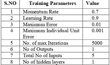
Table 2: Training Parameters For Neural Network Model

S.NO Training Parameters Value

1 Momentum Rate 0.7 2 Learning Rate 0.9 3 Maximum Error 0.01 4 Maximum Individual Unit

Error

0.001

5 No. of max Iterations 5000 6 No of Outputs 1 7 Total No of Inputs 5 8 No of hidden layers 1

Name Error Old

weight

η*E*x New

weight Nw14 -0.00006 0.2 -0.00006 0.1999

Nw15 -0.00027 0.7 -0.00027 0.6997

Nw24 -0.00006 -0.1 -0.00018 -0.1002

Nw25 -0.00027 -1.2 -0.0008 1.2008

Nw34 -0.00006 0.4 -0.00012 0.3998

Nw35 -0.00027 1.2 -0.00054 1.1995

Nw41 0.0469 1.1 0.00470 1.1047

Nw42 -0.0394 3.1 -0.00393 3.0961

Nw51 0.0469 0.1 0.00003 0.10003

(6)

Table 32: Training Of The Neural Network Model Showing NSE

Input sample

NSE: Normalized System Error Neur on 1 Neuron 2 Neuron 3 Neuron 4 Neuron 5

10 0.00

6701 0.0078 34 0.0081 57 0.0075 85 0.0098 86

20 0.00

9998 0.0099 82 0.0088 38 0.0099 91 0.0092 57

30 0.00

9979 0.0099 63 0.0099 33 0.0099 62 0.0099 99

40 0.00

9980 0.0097 65 0.0099 71 0.0099 25 0.0097 77

50 0.00

9742 0.0098 69 0.0098 30 0.0096 32 0.0095 74

60 0.00

9944 0.0099 18 0.0098 61 0.0097 89 0.0097 40

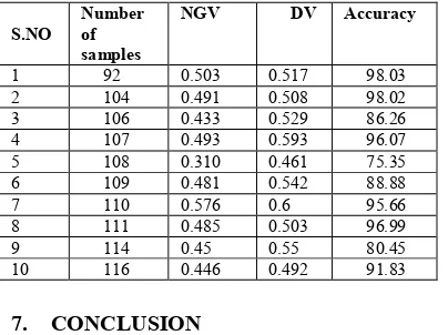
[image:6.612.85.287.353.504.2]

Testing: Accuracy = 100*Network Generated Value (NGV) / Desired Value(DV)

Table 4: Testing The Neural Network Model For Different Samples

7. CONCLUSION

In every day services and applications an artificial neural network models are widely used so that there is a need to understand theory that stands behind them. Artificial neural networks have been find in working areas such as process control, chemistry, gaming, radar systems, automotive industry, space industry, astronomy, genetics, banking, fraud detection, etc. and determine the issues such as approximation functions, analysis of linear and multi variant regression problems, prediction based on time series, problems on classification methods, pattern recognition, decision making process, data processing methods, filtering techniques, clustering formation etc. In this paper, artificial neural networks are briefly introduced and focus the architectures of single layer (SFNN) and multi layer feed forward neural networks (MLFFNN) to learn the theory behind the topologies with detailed examples. After describing

various types of artificial neural networks architectures, the optimization is shown by executing the back propagation neural network model in c programming software.

REFERENCES:

[1] Vidyullatha p, D Rajeswara Rao, Lakshmi Prasanna, “A Conceptual Framework For Approaching Predictive Modeling Using Multivariate Regression Analysis Vs Artificial Neural Network” Journal of Theoretical and

Applied Information Technology, 20th July

2015. Vol.77. No.2, pgno: 287-290, ISSN: 1992-8645 www.jatit.org E-ISSN: 1817-3195. [2] Vidyullatha pellakuri , D. Rajeswara Rao,

“Applying Regression Technique On Environmental Data By WEKA”, International

Journal of Applied Engineering Research,

ISSN 0973-4562 Volume 10, Number 2 (2015) pp. 4619-4626, http://www.ripublication.com. [3] Fardis NAKHAEI, Mehdi IRANNAJAD

“Comparison Between Neural Networks And Multiple Regression Methods In Metallurgical Performance Modeling Of Flotation Column”, Physicochem. Probl. Miner. Process. 49(1), 2013, 255−266, www.minproc.pwr.wroc.pl/journal/

[4] Anyaeche C. O., Ighravwe D. E. “Predicting performance measures using linear regression and neural network: A comparison”, African Journal of Engineering Research, Vol. 1(3), pp. 84-89, July 2013

[5] Asghar Azizi, Seyyed Zioddin Shafaei, Reza Rooki, Ahmad Hasanzadeh, Mostafa Paymard, “Estimating of gold recovery by using back propagation neural network and multiple linear regression methodsin cyanide leaching process”, Materials Science, An Indian Journal Trade Science Inc. MSAIJ, 8(11), 2012 [443-453], ISSN : 0974 – 7486 Volume 8 Issue 11. [6] Maitha H. Al Shamisi, Ali H. Assi and Hassan

A. N. Hejase “Using MATLAB to Develop Artificial Neural Network Models for Predicting Global Solar Radiation in Al Ain City – UAE” United Arab Emirates University, 2010, www.intechopen.com

[7] In 2008, Gang Sun, Steven J. Hoff, Brian C. Zelle, Minda A. Smith, “Development and Comparison of Backpropagation and Generalized Regression Neural Network Models to Predict Diurnal and Seasonal Gas and PM 10 Concentrations and Emissions from Swine Buildings”, Transactions of the ASABE Vol. 51(2): 685-694, American Society of

S.NO

Number of samples

NGV DV Accuracy

1 92 0.503 0.517 98.03

2 104 0.491 0.508 98.02

3 106 0.433 0.529 86.26

4 107 0.493 0.593 96.07

5 108 0.310 0.461 75.35

6 109 0.481 0.542 88.88

7 110 0.576 0.6 95.66

8 111 0.485 0.503 96.99

9 114 0.45 0.55 80.45

(7)

Agricultural and Biological Engineers ISSN 0001-2351 685

[8] Grivas, G., and A. Chaloulakou 2006, “Artificial neural network models for prediction of PM10 hourly concentrations in the greater area of Athens, Greece”, Atmos. Environ. 40(7):1216‐1229.

[9] Haykin, S. (2000), "Neural Networks”, Second Edition, Addison Wesely Longman.

[10] Zurada, J., Introduction to Artificial Neural Systems, West Publishing Company, 1992, digitized 17 nov 2007, publisher West, 1992 [11] Ben Krose and Patrick van der Smagt (1996),