Essays on the term structures of bonds and equities

Essays on the Term Structures of

Bonds and Equities

Wen Yan

Thesis submitted to the Department of Finance

of the London School of Economics for the degree of PhD in Finance

I certify that the thesis I have presented for examination for the PhD degree of the London School of Economics and Political Science is solely my own work other than where I have clearly indicated that it is the work of others (in which case the extent of any work carried out jointly by me and any other person is clearly identified in it).

The copyright of this thesis rests with the author. Quotation from it is permitted, provided that full acknowledgement is made. This thesis may not be reproduced without my prior written consent.

I warrant that this authorisation does not, to the best of my belief, infringe the rights of any third party.

Chapter 1 “The Term Structure of Equities” examines the term structure of equities. Using observed prices of dividend strips, prices of zero-coupon equities are extracted, and their yields and returns characteristics are documented. An affine term structure model is used to model the term structure of equities. The model is estimated, and model-implied equity yields and returns are shown to match the data well. However, the model-implied long-run risk-neutral mean of the short rate is implausible. (The next chapter takes this into account and estimates bond and equity yield curves jointly using data on both zero-coupon bonds and zero-coupon equities.)

Abstract

Acknowledgment

1. The Term Structure of Equities

1.1 Abstract . . . 14

1.2 Introduction . . . 14

1.3 The model . . . 17

1.4 Estimation . . . 23

1.5 Conclusion . . . 49

2. Estimating a Unified Framework of Co-Pricing Stocks

and Bonds

2.2 Introduction . . . 50

2.3 Model and estimation . . . 55

2.4 Restricted Model . . . 67

2.5 Conclusion . . . 75

3. The Role of Asian Countries’ Reserve Holdings on

the International Yield Curves

3.2 Introduction . . . 76

3.3 Data . . . 80

factors . . . 92 3.5 Estimation . . . 96 3.6 Conclusion . . . 113

Appendix 1

A1.1 Solutions for asset prices . . . 120 A1.2 Proof of Proposition 1 . . . 123 A1.3 Proof of Proposition 2 . . . 126

Appendix 2

1.1 Short rate, in annual percentages, 1996m2:2009m10 . . . 32

1.2 Monthly dividends and log dividend growth rates, original and filtered. . . 34

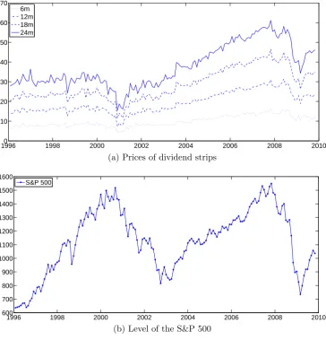
1.3 Prices of dividend strips and the level of the S&P 500, 1996m1:2009m10 . . . 37

1.4 Prices of zero-coupon equities, 1996m1:2009m10 . . . 40

1.5 Annual percentage yields of zero-coupon equities . . . 41

1.6 First principal component of zero-coupon equities . . . . 41

1.7 Estimated risk premiums of zero-coupon equities, equity term structure . . . 48

2.1 Zero-coupon bond yields, 1996m2:2009m10 . . . 58

2.2 Estimated risk premiums of zero-coupon equities, unre-stricted co-pricing model . . . 65

2.3 Estimated risk premiums of zero-coupon equities, restricted co-pricing model . . . 73

3.1 Annual % bond yields, United States . . . 81

3.2 Annual % bond yields, United Kingdom . . . 82

3.3 Annual % bond yields, Germany . . . 82

3.4 Annual % bond yields, Canada . . . 83

3.5 Annual % bond yields, Switzerland . . . 83

3.6 Annual % bond yields, Australia . . . 83

3.7 Reserve holdings of Asian countries, including China, Japan and South Korea, in billions of U.S. dollars . . . 87

3.8 Annual % GDP growth and inflation, United States . . . 89 3.9 Annual % GDP growth and inflation, United Kingdom . 90 3.10 Annual % GDP growth and inflation, Germany . . . 90 3.11 Annual % GDP growth and inflation, Canada . . . 91 3.12 Annual % GDP growth and inflation, Switzerland . . . . 91 3.13 Annual % GDP growth and inflation, Australia . . . 92 3.14 Impulse response functions of yields to a one standard

de-viation shock to Asian reserves. Impulse responses for yields of maturities of one quarter (top panel), four quar-ters (middle panel) and twenty quarquar-ters (bottom panel), United States . . . 99 3.15 Impulse response functions of yields to a one standard

de-viation shock to Asian reserves. Impulse responses for yields of maturities of one quarter (top panel), four quar-ters (middle panel) and twenty quarquar-ters (bottom panel), United Kingdom . . . 103 3.16 Impulse response functions of yields to a one standard

de-viation shock to Asian reserves. Impulse responses for yields of maturities of one quarter (top panel), four quar-ters (middle panel) and twenty quarquar-ters (bottom panel), Germany . . . 106 3.17 Impulse response functions of yields to a one standard

3.18 Impulse response functions of yields to a one standard de-viation shock to Asian reserves. Impulse responses for yields of maturities of one quarter (top panel), four quar-ters (middle panel) and twenty quarquar-ters (bottom panel), Switzerland . . . 110 3.19 Impulse response functions of yields to a one standard

1.1 Maximum likelihood estimates of the risk-neutral param-eters, equity term structure . . . 42 1.2 Maximum likelihood estimates of the conditional

covari-ance, equity term structure . . . 42 1.3 Maximum likelihood estimates of the physical parameters,

equity term structure . . . 43 1.4 Estimation results: moments comparison for equity yields,

annual percentages, equity term structure . . . 44 1.5 Data: summary statistics of the return of the short-term

strip and the market, annual percentages . . . 44 1.6 Summary statistics of the return of the short-term strip

and the market, equity term structure, annual percentages 46 1.7 Summary statistics of the excess return of the short-term

strip and the market, equity term structure, annual per-centages . . . 46 2.1 Summary statistics of the U.S. bond yields (all numbers

are in annualized percentages) . . . 58 2.2 Maximum likelihood estimates of the risk-neutral

param-eters, unrestricted co-pricing model . . . 60 2.3 Maximum likelihood estimates of the conditional

covari-ance, unrestricted co-pricing model . . . 60 2.4 Maximum likelihood estimates of the physical parameters,

unrestricted co-pricing model . . . 61

2.5 Estimation results: moments comparison for equity yields, annual percentages, unrestricted co-pricing model . . . . 62 2.6 Data: summary statistics of the return of the short-term

strip and the market . . . 62 2.7 Summary statistics of the return of the short-term strip

and the market, unrestricted co-pricing model . . . 63 2.8 Summary statistics of the excess return of the short-term

strip and the market, unrestricted co-pricing model . . . 63 2.9 Estimation results: moments comparison for zero-coupon

bonds (all numbers are in annualized percentage), unre-stricted co-pricing model . . . 66 2.10 Maximum likelihood estimates of the risk-neutral

param-eters, restricted co-pricing model . . . 68 2.11 Maximum likelihood estimates of the conditional

covari-ance, restricted co-pricing model . . . 69 2.12 Maximum likelihood estimates of the physical parameters,

restricted co-pricing model . . . 70 2.13 Estimation results: moments comparison for equity yields,

annual percentages, restricted co-pricing model . . . 71 2.14 Summary statistics of the return of the short-term strip

and the market, restricted co-pricing model . . . 71 2.15 Summary statistics of the excess return of the short-term

strip and the market, restricted co-pricing model . . . 72 2.16 Estimation results: moments comparison for zero-coupon

bonds (all numbers are in annualized percentage), restricted co-pricing model . . . 74 3.1 Summary statistics of the international bond yields (all

country . . . 87 3.3 Regressions of excess returns on ten-year bonds on yield

factors and macro factors; Newey–West standard errors with four lags are shown in parentheses. . . 88 3.4 Variance decompositions, United States . . . 101 3.5 Proportion of yields’ forecast variance explained by macro

factors (reserves, GDP growth, inflation) and reserves, United States . . . 101 3.6 Proportion of yields’ forecast variance explained by macro

factors (reserves, GDP growth, inflation) and reserves, United Kingdom . . . 105 3.7 Proportion of yields’ forecast variance explained by macro

factors (reserves, GDP growth, inflation) and reserves, Germany . . . 107 3.8 Proportion of yields’ forecast variance explained by macro

factors (reserves, GDP growth, inflation) and reserves, Canada . . . 109 3.9 Proportion of yields’ forecast variance explained by macro

factors (reserves, GDP growth, inflation) and reserves, Switzerland . . . 111 3.10 Proportion of yields’ forecast variance explained by macro

The Term Structure of Equities

1.1

Abstract

This chapter examines the term structure of equities. Using observed prices of dividend strips, prices of zero-coupon equities are extracted, and their yields and returns characteristics are documented. An affine term structure model is used to model the term structure of equities. The model is estimated, and model-implied equity yields and returns are shown to match the data well. However, the model-implied long-run risk-neutral mean of the short rate is implausible. (The next chapter takes this into account and estimates bond and equity yield curves jointly using data on both zero-coupon bonds and zero-coupon equities.)

1.2

Introduction

There is an extensive literature on identifying the common factors that affect the bond yield curve. The work by Litterman and Scheinkman (1991) showed that three factors, namely “level”, “slope” and “curva-ture”, explain over 90% of cross-sectional bond yield variations for al-most any reasonable length of sample period and any combination of yield maturities. This result is so robust that factor analysis has since populated the analysis of bond term structure, with a fourth factor coined by Cochrane and Piazzesi (2005), namely “the return forecasting factor”, and the discovery of the “hidden factor” by Duffee (2011).

yield curve, the equity yield curve is rarely studied. The literature has mostly focused on studying the risk and return behavior of the aggregate stock market without looking at the individual terms that comprise it. However, because the value of the aggregate stock market can be viewed as the total value of the discounted future dividend payments (Gordon 1962), in addition to studying the aggregate price of these dividend pay-ments, exploring the properties of each dividend payment should provide us with valuable information about the way stock prices are formed and improve our understanding of investors’ risk preferences and the endow-ment or technology process in macro-finance models. Hence in this paper, I study the term structure of equities by exploring the properties of the individual dividend payments that comprise the aggregate stock mar-ket. More specifically, I focus on zero-coupon equities, a concept created using the analogy of zero-coupon bonds. Just like a zero-coupon bond giving the investor a fixed payment at the end of the bond’s maturity, a zero-coupon equity simply gives the investor a variable payment, that is, the stochastic dividend, at the end of the security’s maturity. This stochastic dividend could be paid out by a particular company, industry or the aggregate economy. And the sum of discounted future dividend payments will be the value of the company, industry or the aggregate economy. In this paper, I focus on the term structure of the stochastic dividends of varying maturities paid out by the aggregate stock market index. And the first important questions for us are what the yield and return characteristics of the zero-coupon equities are and whether there exist common factors that can price the equity yield curve well.

earlier) – these are often available for maturities from one month to 30 years. But such data has not been available for equities. However, my study of the equity term structure is made possible by the availability of dividend strips data on the S&P 500 from van Binsbergen, Brandt and Koijen (2012). Specifically, whereas a zero-coupon equity of maturity

n at time t gives the investor a stochastic dividend payment from t+

n−1 to t+n, buying a dividend strip of maturity n at time t entitles the investor to all the dividends paid out from time t to t +n. Using put–call parity and observed put and call prices on the S&P 500, i.e. Long-Term Equity Anticipation Securities (LEAPS) from the Chicago Board Options Exchange (CBOE), van Binsbergen, Brandt and Koijen decompose the index into a long-term equity and a short-term equity, which is the dividend strip. In particular, prices of dividend strips for maturities of six, twelve, eighteen and twenty-four months are priced, and I extract zero-coupon equity prices from the prices of these strips.

By estimating the term structure of equities, this paper fills the gap in the literature in which only the term structure of bonds was estimated. Both Lettau and Wachter (2007) and Lettau and Wachter (2011) study the equity term structure, but they do not use data on zero-coupon eq-uities or dividend strips. Moreover, what we learn using an estimated factor model is that we can see from the data the dynamics among factors. The calibration exercise usually makes strong and sometimes counterfac-tual assumptions on the dynamics of factors and the interaction between them. For example, in Lettau and Wachter (2011), dividend growth fol-lows an autoregressive process with positive autocorrelation coefficient. However, in the data, dividend growth is strongly negatively autocorre-lated. Such restrictions will likely distort the model’s predictions of asset prices and each factor’s implication on the asset prices.

The rest of the chapter is structured as follows: Section 1.3 outlines the affine term structure model that is able to price zero-coupon eq-uities, the aggregate stock market index as well as zero-coupon bonds. Section 1.4 describes the data, estimation strategy and estimation results and shows the model implications for bond yields. Section 1.5 concludes.

1.3

The model

equity pricing. And the way of using affine term structure techniques to value zero-coupon equities for each maturity and summing over the prices of zero-coupon equities of all maturities to reach the aggregate market index has been applied in Ang and Liu (2004), Bekaert, Engstrom and Grenadier (2010), Lettau and Wachter (2007), Lettau and Wachter (2011) and Wachter (2006).

1.3.1

The economy

It is assumed that the economy at time t is driven by a state vector Xt

that follows a VAR(1) process under both the physical measure _P and the risk-neutral measure _Q,

∆Xt=K0PX +K1PXXt−1+ ΣXPt, (1.1)

∆Xt=K0QX +K1QXXt−1+ ΣXQt, (1.2)

where Xt is an N ×1 vector, K0PX and K0QX are N ×1 vectors, K1PX,

KQ

1X and ΣX are N ×N matrices and both Pt and Qt are N×1 vectors

of independent shocks to various risk factors affecting the economy with mean zero and unit variance.

Let rt = logRt, the one-period interest rate, be an affine function of

the state vector,

rt =ρ0X +ρ01XXt, (1.3)

where ρ0X is a scalar and ρ1X is an N ×1 vector.

The level of the aggregate dividend of the economy is denoted by Dt.

Letdt= logDt, and the log dividend growth rate from timet−1 to time

t be defined as ∆dt = log(Dt/Dt−1). To maintain the affine structure

function of the underlying state vector, i.e.

∆dt =δ0X +δ10XXt, (1.4)

where δ0X is a scalar and δ1X is an N ×1 vector.

Let the market price of risk vector λt be affine in the state vector,

λt=λ0X +λ1XXt. (1.5)

Here λt is an N ×1 vector of time-varying market prices of risk, λ0X is

anN ×1 vector and λ1X is an N ×N matrix.

By no-arbitrage, we obtain the pricing kernel or the stochastic dis-count factor (SDF) Mt+1 of the economy as

Mt+1 = exp(−rt−1₂λt0λt−λ0tt+1), (1.6)

which can be used to consistently price all assets. That is, we have the Euler equation

1 =Et[Mt+1Rt+1], (1.7)

where Rt+1 is the one-period return on any asset in the economy.

1.3.2

Zero-coupon equities

form that is similar to the price of the zero-coupon bond. Specifically, let Pd

nt denote the time-t price of a zero-coupon equity of

maturity n, that is, the time-t price of the aggregate dividend paid out between time t+n−1 and time t+n. This implies that its one-period return from t to t+ 1 can be written as

R_n,td ₊₁ = P

d

n−1,t+1

Pd

n,t

= P

d

n−1,t+1/Dt+1

Pd

n,t/Dt

Dt+1

Dt

. (1.8)

Plugging this into the Euler equation implies that the price scaled by the aggregate dividend will satisfy the following equation:

Pd

nt

Dt

=Et

Mt+1

Pd

n−1,t+1

Dt+1

Dt+1

Dt

. (1.9)

If we write the scaled equity price as an exponential affine function of the state vector, i.e.

Pd

nt

Dt

= exp(Ad_n+B_nd0Xt), (1.10)

then all quantities in the Euler equation can now be expressed as expo-nential affine functions of the state vector. Moreover, using the Euler equation, we can express the constantAd

n and the 1×N loadings of the

scaled equity price on the state vector, i.e. Bd

n

0

, as functions of the un-derlying parameters of the model by solving a set of Riccati equations with the boundary condition Pd

0t/Dt= 1.

More specifically, the loadings are solved recursively as follows:

Ad_n=−(ρ0X −δ0X) +Adn−1+ (δ1X +Bnd−1) 0

KQ

0X

+ 1₂(δ1X +Bnd−1) 0

ΣXΣ0X(δ1X +Bnd−1), (1.11)

B_nd0 =−ρ0_1X + (δ1X +Bnd−1) 0

(KQ

with the starting values of Ad

0 = 0 and B0d = 0. Details of the derivation

are provided in Appendix A1.1. Moreover, we have

y_ntd =−1

nln Pd

nt

Dt

=−1

n(A

d

n+B

d

n

0

Xt) = −

1 nA d n− 1 nB d n 0

Xt. (1.13)

When we use the affine model to price bonds, bond yields are affine functions of the state vector, and in estimation we try to match the estimated bond yields with the observed bond yields. Analogously, when we use the affine model to price equities, the quantity

y_ntd =−1

nln Pd

nt

Dt

will be the equity “yield” that we try to match.

1.3.3

The aggregate market

Since a zero-coupon equity is an asset that pays off the aggregate dividend at some fixed maturity, by summing the prices of zero-coupon equities of all maturities, we get the aggregate market index. Note here that, unlike the prices of zero-coupon equities, which are exponential affine functions of the state vector, the market index will not be an exponential affine function of the state vector

P_tm=

∞

X

n=1

P_ntd =

∞

X

n=1

exp(Ad_n+B_nd0Xt)×Dt. (1.14)

1.3.4

Zero-coupon bonds

for completeness and convenience, the pricing equations of zero-coupon bonds are outlined here. To price nominal bonds, let Pb

nt denote the

time-t price of the n-period nominal zero-coupon bond. Assuming bond price is exponential affine in the state vector

P_ntb = exp(Ab_n+B_nb0Xt), (1.15)

where Ab

n is a scalar and Bnb is an N ×1 vector, by the Euler equation

we have

P_ntb =Et[Mt+1Pnb−1,t+1] (1.16)

with the boundary condition P₀b_t= 1. The price of the zero-coupon bondPb

nt = exp(Abn+Bnb

0

Xt) has exactly

the same form as the scaled price of the zero-coupon equity, which is

Pd

nt/Dt= exp(Adn+Bnd

0

Xt). And the Euler equation for the zero-coupon

bond is exactly the same as the Euler equation for the zero-coupon equity without the dividend growth process. Hence we can just take the results from the zero-coupon equity, set δ0X = 0 and δ1X = 0 and change the

superscript from d to b to get the standard solutions for bond prices’ loadings on the state vector, which are

Ab_n =−ρ0X +Abn−1+Bnb−1 0

KQ

0X +

1 2B

b

n−1 0

ΣXΣ0XB

b

n−1, (1.17)

B_nb0 =−ρ0_1X +B_nb₋₁0(KQ

1X +I), (1.18)

with the starting values being Ab

n= 0 andBnb= 0.

And bond yield of maturity n can be expressed as

y_ntb =−1

n lnP

b

nt =−

1

n(A

b

n+B

b

n

0

Xt) =−

1 nA b n− 1 nB b n 0

1.4

Estimation

1.4.1

The normalized model

The general Gaussian dynamic term structure model previously stated in Section 1.3 is not ready to be estimated, as any affine transformations of the state process are observationally equivalent as shown in Dai and Singleton (2000). That is, suppose we have two models; they are the same in all aspects except that the state process in one model is an affine transformation of the state process in the other model. Then the two models will generate exactly the same asset prices. In other words, given the same set of asset prices, there exists an infinite number of models that can generate this set of asset prices. Therefore, these models are generally not identified without imposing restrictions. To impose the minimum number of restrictions on the state process such that the model is identified, we can follow Joslin, Singleton and Zhu (2011) (JSZ) and normalize all models to a canonical form, in which the state vector Xt

is entirely latent. As a result of this normalization, given the same set of asset prices, there is only one model in the canonical form that can generate this set of asset prices. The JSZ canonical form is only able to price zero-coupon bonds. I extend the canonical form in JSZ to a canonical form that is able to price zero-coupon equities as well.

Let us first recall the general form of the state process in Section 1.3, in which the parameters are unrestricted:

∆Xt=K0PX +K1PXXt−1+ ΣXPt,

∆Xt=K0QX +K Q

1XXt−1+ ΣXQt,

rt=ρ0X +ρ01XXt,

∆dt=δ0X +δ10XXt,

where ΣXΣ0X is the constant conditional covariance matrix ofXt,Pt, Qt ∼

N(0, IN), rt is the short rate, ∆dt is the dividend growth.

Next, as this model belongs to the class of Gaussian dynamic term structure models, it is observationally equivalent up to an affine trans-formation of the state vector. Hence, using this feature, we can derive a canonical form of the above general co-pricing model, which is maxi-mally flexible in the parameterization of both its _P and _Q distributions of Xt such that the model is identifiable. Here, no assumptions about

the processes of Xt are made; only normalizations are used to ensure

econometric identification. Proposition 1 shows the canonical form, and the proof is given in Appendix A1.2.

Proposition 1. Every canonical affine term structure model is ob-servationally equivalent to the following canonical model:

∆Xt=K0PX +K1PXXt−1+ ΣXPt,

∆Xt=K₀Q_X +K₁Q_XXt−1+ ΣXQt,

rt=r∞Q +ι 0

Xt,

∆dt=δ0X +δ10XXt,

(1.21)

where P

t, Qt ∼ N(0, IN), K₀Q_X = 0, K₁Q_X is in ordered real Jordan form1

such that the diagonal elements are represented by λQ _{= (λ}Q

i )s with

de-creasing magnitude, ΣX is the lower triangular Cholesky decomposition

of ΣXΣ0X,ι is a vector of ones.

The result of this proposition will be used in the estimation to make sure the model is not unidentified or has any over-identifying restrictions.

1_{Alternatively,K}Q

1Xcan be specified to be a diagonal matrix with real and distinct

1.4.2

Estimation strategy

One way to estimate the model is to maintain the assumption that the underlying state vector is completely latent as in (1.21). However, one problem with this estimation strategy is that the number of parameters that need to be estimated can potentially be very large.

An alternative estimation strategy is to estimate _P parameters and

Q parameters separately, as in Joslin, Singleton and Zhu (2011). It is

shown below that the canonical model in terms of Xt is observationally

equivalent to a unique affine model whose pricing factors Pt include the

short rate, the first principal component of the set of equity yields that can be viewed as a portfolio of equity yields, and the dividend growth. Under the assumption that the portfolio of yields is observed without error, the estimation of the canonical model in terms ofPtcan be carried

out in a two-step procedure. First, the _P dynamics of the state process can be estimated by an unrestricted vector autoregression (VAR). Then, taking the estimated parameters from the VAR as given, the rest of the parameters are then estimated using maximum-likelihood estimation (MLE). The advantage of this estimation procedure is that the number of parameters to be estimated is greatly reduced. Therefore, the latter strategy will be adopted in this paper.

Specifically, I assume there are three latent factors driving the econ-omy. Applying rotation to the latent state vector, it can be shown that the canonical model in terms of Xt defined in (1.21) is observationally

equivalent to a canonical model defined in terms of Pt, which consists of

the short rate, the first principal component of equity yields (portfolio of yields)

and dividend growth, i.e.

Pt =       rt PCt

∆dt       . Given

yt=AX +BX0 Xt, (1.23)

we have

Pt=       rt PCt

∆dt       =      

ρ0X

W AX

δ0X       +      

ρ0_1X W B_X0

δ₁0_X

     

Xt=A+BXt. (1.24)

Therefore, given the affine relationship betweenPtandXt, we can use the

generic feature of Gaussian affine term structure models to find a model in terms of Pt, which is observationally equivalent to the canonical form

of Xt. This is summarized in Proposition 2. The proof can be found in

Appendix A1.3.

Proposition 2. Any canonical affine term structure model as defined in (1.21) is observationally equivalent to a unique affine co-pricing model whose pricing factors Pt include the short rate, the portfolios of yields

W yt and the dividend growth. Moreover, the Q distribution of Pt is

uniquely determined by (λQ_{, r}Q

ordered in decreasing magnitude. That is,

∆Pt=K0PP +K1PP Pt−1+ ΣPP_t,

∆Pt=K0PQ +, K1PQ Pt−1+ ΣPQt

rt=ρ0P +ρ01PPt,

∆dt=δ0P+δ1P0 Pt

(1.25)

is a canonical Gaussian affine term structure model, where KP

0P, K1PP ,

ρ0P, ρ1P, δ0P, δ1P are explicit functions of (λQ, rQ∞, ΣP, δ0X, δ1X). The

canonical form is parameterized by (λQ_{, r}Q

∞, ΣP, δ0X, δ1X, K0PP , K1PP ).

And the relationship between the parameters in the two canonical forms can be shown as follows:

KQ

1P =BJ(λQ)B −1_,

KQ

0P =−K1PQ A,

ρ1P = (B−1)0ι,

ρ0P =rQ∞−A0ρ1P,

δ1P = (B−1)0δ1X,

δ0P =δ0X −A0δ1P.

(1.26)

Next given the observational equivalence between the canonical form in Xt and the model in Pt outlined above, I estimate the model in Pt

rather than in Xt. The estimation is implemented in three steps.

In Step 1, I assume there is one portfolio of yields that is measured without error, i.e. W yt = W yot. Here, yot denotes the observed yields.

In Step 2, as the state vector

Pt =       rt PCt

∆dt      

is observed, it can be used to estimate the _P process of Pt. More

specif-ically, as Pt follows a VAR process

∆Pt =KP

0P+K1PP Pt−1+ ΣPPt,

KP

0P andK1PP can be estimated from an unrestricted VAR using ordinary

least squares (OLS). And these OLS estimates can be viewed as MLE estimates because of the inherent separation between the parameters of the _P and _Q dynamics of Pt, that is

f(y_to|y_to₋₁; Θ) =f(yo_t|Pt;λQ, r∞Q,ΣP, δ0X, δ1X, Pθm)

×f(Pt|Pt−1;K1PP , K0PP ,ΣP), (1.27)

wherePθm _{is the conditional distribution of the measurement errorsy}o

t−

yt.

In Step 3, taking the estimated parameters from OLS as given, we estimate the rest of the parameters using MLE.

The detailed justification for the estimation strategy is as follows. By Proposition 2, we can, without loss of generality, use

Pt=       rt PCt

∆dt      

as observed factors. Suppose that the individual bond yields, yt, are

to be used in estimation and that their associated measurement errors,

yo

t−yt, have the conditional distributionPθm, for someθm ∈Θm. It only

requires that, for any Pθm_{, these errors are conditionally independent}

of lagged values of the measurement errors and satisfy the consistency condition P             rt

W yo

t

∆dt       =       rt PCt

∆dt       |Pt      

= 1.

Then the conditional likelihood function (under _P) of the observed data (y_to) can be decomposed as the product of two conditional likelihood func-tions. The first likelihood function describes the conditional distribution of the observed yields that are measured with errors, that is, dependent on the parameters relevant for pricing (λQ_,rQ

∞, ΣP,δ0X,δ1X) and the

dis-tribution assumption of the measurement errors. The second likelihood function describes the conditional distribution ofPt, which depends only

on (KP

1P, K0PP , ΣP). We have

f(y_to|y_to₋₁; Θ) =f(yo_t|Pt;λQ, r∞Q,ΣP, δ0X, δ1X, Pθm)

×f(Pt|Pt−1;K1PP , K0PP ,ΣP).

Now if we assume Pt is conditionally Gaussian, then the conditional

P likelihood of P, i.e. the second part of (1.28) can be expressed as

f(Pt|Pt−1;K1PP , K0PP ,ΣP)

= (2π)−N/2|ΣP|−1×exp(−1₂

Σ−1_P (P_t−E_t[P_t])

2

), (1.28)

Moreover, Zellner (1962) shows that, conditional on t = 0 informa-tion, the parametersKP

1P andK0PP that maximize this likelihood function

are their OLS estimates, i.e.

(KP

1P, K0PP ) = argmax

T X

t=1

f(y_to|y_to₋₁;KP

1P, K0PP ,ΣP)

= argmin

T X

t=1

Σ−1_P (P_t−E_t[P_t])

2

. (1.29)

Hence, (KP

1P, K0PP ) can be estimated from time series of Pt alone, and

their OLS estimates are globally optimal, i.e. they are equal to their maximum likelihood estimates. Hence (KP

1P,K0PP ) will no longer need to

be estimated using MLE, and the canonical form in P is now parame-terized by (λQ_{, r}Q

∞, ΣP, δ0X,δ1X) rather than by (λQ,r∞Q, ΣP, δ0X, δ1X,

KP

0P, K1PP ), effectively eliminating the dependence on (K1PP , K0PP ). The

separation is formally shown in Proposition 3.

Proposition 3. Using the observed factor, Pt = Pto ∈ RN, the

maximum likelihood estimates of (KP

1P, K0PP ) are given by their OLS

estimates. Moreover, the canonical form of Pt in Proposition 2 is now

parameterized by (λQ_{, r}Q

∞, ΣP, δ0X, δ1X), effectively eliminating the

de-pendence on (KP

1P, K0PP ).

Moreover, the sample estimates of ΣP can be used as starting values

for their MLE estimation, reducing the estimation time of these param-eters. The reduction in the number of parameters need to be estimated using MLE increases with the number of factors that are assumed to drive the economy. For example, with an N-factor model, we no longer need to estimate the N(N + 1) parameters that come from (KP

1P,K0PP ),

1.4.3

Data

This subsection describes the data used in this paper, especially the three observed factors assumed to drive the whole economy, i.e. the short rate, dividend growth and portfolio of equity yields. The procedure used to remove seasonality in the data and the way the equity portfolio is constructed are also discussed.

Short rate

19960 1998 2000 2002 2004 2006 2008 2010 1

2 3 4 5 6 7

BBK data, short rate, annual percentages, 1996m2:2009m10

Figure 1.1: Short rate, in annual percentages, 1996m2:2009m10

Dividend and dividend growth

Monthly dividends from January 1996 to October 2009 are provided by van Binsbergen, Brandt and Koijen (2012). The dashed line in the top panel of Figure 1.2 shows monthly dividends and the dashed line in the middle panel shows the monthly log dividend growth rates. We can see that the level of dividend is nonstationary but log dividend growth rates are stationary. However, monthly dividends exhibit seasonality in both level and log growth rates, due to the fact that most companies pay dividends on a quarterly basis.

filtering out seasonality can also help us see more clearly the underlying trend of the data.

1996 1998 2000 2002 2004 2006 2008 2010 0.5

1 1.5 2 2.5 3 3.5 4

Orignal dividend Filtered dividend

(a) Monthly dividends,Dt, original and filtered, 1996m1:2009m10

1996 1998 2000 2002 2004 2006 2008 2010 −1

−0.8 −0.6 −0.4 −0.2 0 0.2 0.4 0.6 0.8 1

Orignal dividend growth

(b) Monthly log dividend growth rates, ∆dt = log(Dt/Dt−1), original,

1996m2:2009m10

1996 1998 2000 2002 2004 2006 2008 2010 −0.15

−0.1 −0.05 0 0.05 0.1 0.15 0.2 0.25

Filtered dividend growth

(c) Monthly log dividend growth rates, ∆dt = log(Dt/Dt−1), filtered,

1996m2:2009m10

Equity yield portfolio

Finally, an “equity yield portfolio” is included as a state factor in the estimation. The factor is the first principal component of equity yields, which is a linear combination of equity yields and hence can be viewed as a portfolio of equity yields. Equity yields in this paper are defined by equation (1.13), i.e.

yd_nt =−1

nln Pd

nt

Dt

.

Pd

nt is the price of zero-coupon equities and the data on zero-coupon

19960 1998 2000 2002 2004 2006 2008 2010 10

20 30 40 50 60 70

Prices of dividend strips, in logs, 1996m1:2009m10

6m 12m 18m 24m

(a) Prices of dividend strips

1996 1998 2000 2002 2004 2006 2008 2010 600

700 800 900 1000 1100 1200 1300 1400 1500 1600

Level of the S&P 500, data and fitted, 1996m1:2009m10

S&P 500

(b) Level of the S&P 500

Figure 1.3: Prices of dividend strips and the level of the S&P 500, 1996m1:2009m10

but will nevertheless be large for the market index. Hence, in practice, matching the market index under the affine model will be too compu-tationally intensive. Alternatively, given the fact that the entire strip price curve is generated, we can extract yields directly from the curve. We could use the fitted curve to extract information regarding the long end of the equity term structure. More specifically, a zero-coupon equity of a long-maturity (fifty-year) yield could be taken from the estimated nonlinear curve and be used as the data on the long-maturity yield in the estimation. This equity yield at long maturity will not be a perfect substitute for the market index, but it will nevertheless contain informa-tion on the long end of the equity term structure. By having the equity yield at long maturity, the estimation will have a greater ability to fit the observed market index.

By subtracting the fitted strip prices of two adjacent maturities, we obtain the prices of the zero-coupon equities. The prices of zero-coupon equities (6m, 12m, 18m, 24m and 50y) from January 1996 to October 2009 are plotted in the top panel of Figure 1.4. We can see that the prices of zero-coupon equities follow the same trend as those of dividend strips. And because the four zero-coupon equities’ maturities are close to each other, their prices are generally at the same level. As pointed out by van Binsbergen, Brandt and Koijen (2012) (BBK), dividend strip prices are nonstationary over time; they scale the four dividend strip prices by the level of the S&P 500 index to obtain stationary data series. Indeed, the prices of the zero-coupon equities are nonstationary, as seen from the top panel of Figure 1.4. However, if we scale zero-coupon equity prices by the dividend provided by BBK, then P_ntd/Dt is stationary, as shown by the

19960 1998 2000 2002 2004 2006 2008 2010 0.5

1 1.5 2 2.5 3

Prices of zero coupon equities, level, 1996m2:2009m10

6m 12m 18m 24m 50y

(a) Prices of zero-coupon equities

19960 1998 2000 2002 2004 2006 2008 2010 0.2

0.4 0.6 0.8 1 1.2 1.4 1.6 1.8

Prices of zero coupon equities, level scaled by original dividend, 1996m2:2009m10

6m 12m 18m 24m 50y

(b) Prices of zero-coupon equities scaled by original dividend

19960 1998 2000 2002 2004 2006 2008 2010 0.2

0.4 0.6 0.8 1 1.2 1.4

Prices of zero coupon equities, level scaled by filtered dividend, 1996m2:2009m10

6m 12m 18m 24m 50y

(c) Prices of zero-coupon equities scaled by filtered dividend

Figure 1.4: Prices of zero-coupon equities, 1996m1:2009m10

and the first principal component explains over 99% of the total varia-tions in this group of equity yields. Figure 1.5 plots the time series of the five yields. The two spikes in 2001 and 2009 are indicative of two economic recessions. Figure 1.6 plots the time series of the first principal component of the equity yields.

1996 1998 2000 2002 2004 2006 2008 2010 −40

−20 0 20 40 60 80 100 120 140

Zero coupon equity yields, annual percentages, 1996m2:2009m10

6m 12m 18m 24m 50y

Figure 1.5: Annual percentage yields of zero-coupon equities

1996 1998 2000 2002 2004 2006 2008 2010 −0.5

0 0.5 1 1.5 2

Figure 1.6: First principal component of zero-coupon equities

1.4.4

Estimation results

Model parameters

As the likelihood function is optimized over (λQ_,rQ

∞, ΣP,δ0X,δ1X), these

are in annual numbers with their standard deviations in parentheses. From the estimates of the (λQ

i + 1)s, we can see that the estimated state

process has real and distinct eigenvalues, and because all (ˆλQ

i + 1)s are

between zero and one, the estimated state process is stationary under

Q. The initial value of ΣP is obtained from the VAR estimate of the P

process of the state vector, and the final estimate of ΣP obtained from

the MLE is reported in Table 1.2. Table 1.3 reports the OLS estimates of KP

0P and K1PP +I.

Table 1.1: Maximum likelihood estimates of the risk-neutral parameters, equity term structure

λQ

1 + 1 λQ2 + 1 λQ3 + 1 rQ∞

Estimate 0.9967 0.3761 0.3068 −670.2887 Standard deviation (0.0010) (0.0170) (0.6789) (0.3190)

δ0X δ1X,1 δ1X,2 δ1X,3

Estimate −6.7241 0.9983 −0.7104 −1.3359 Standard deviation (0.0117) (0.0030) (0.8033) (1.1760)

Table 1.2: Maximum likelihood estimates of the conditional covariance, equity term structure

P P,11

Estimate 0.4655 Standard deviation (0.0304)

P P,21

P P,22

Estimate −0.6509 19.6996 Standard deviation (1.2707) (2.0452)

P P,31

P P,32

P P,33

Table 1.3: Maximum likelihood estimates of the physical parameters, equity term structure

KP

0P,1 K0PP ,2 K0PP ,3

Estimate 0.0585 −2.9820 0.9645 Standard deviation (0.0764) (3.4513) (9.0396)

KP

1P,11+ 1 K1PP ,12 K1PP ,13

Estimate 0.9820 −0.0023 −0.0008 Standard deviation (0.0200) (0.0011) (0.0006)

KP

1P,21 K1PP ,22+ 1 K1PP ,23

Estimate 1.6157 0.7616 −0.0425 Standard deviation (0.9032) (0.0491) (0.0263)

KP

1P,31 K1PP ,32 K1PP ,33+ 1

Estimate 2.6735 −0.5392 −0.2203 Standard deviation (2.3657) (0.1286) (0.0690)

Equity yields

Table 1.4: Estimation results: moments comparison for equity yields, annual percentages, equity term structure

Maturity (years) 0.5 1 1.5 2 long maturity (50) Panel A: Data

Mean 6.91 4.38 3.53 3.11 1.85 Standard deviation 28.60 14.17 9.36 6.96 0.38

Panel B: Model

Mean 6.91 4.38 3.53 3.11 1.85 Standard deviation 28.60 14.21 9.34 6.90 0.10

Return of the dividend strip and the aggregate market

BBK construct the return of the short-term strip and compare it with the return of the market. They find that the return of the short-term strip is much higher than that of the market. Given the return of the market can be viewed as a weighted average of the return of the short-term strip and the return of the long-term strip, the above observation implies that the return of the short-term strip is higher than the return of the long-term strip, i.e. the equity term structure is downward sloping. This can be illustrated by Table 1.5.

Table 1.5: Data: summary statistics of the return of the short-term strip and the market, annual percentages

R_{short strip} R_{short strip}−Rf R_market R_market−Rf

Mean 13.90 10.53 6.67 3.29

Standard 27.03 27.04 16.26 16.22

deviation

Sharpe ratio 0.39 — 0.20 —

the short-term asset is higher than the Sharpe ratio of the market despite its high volatility.

We can also check whether this evidence can be generated by the model in the paper. In particular, the two returns are calculated as follows. For the short-term strip, its return can be calculated as

Rs_t+1 = P

s

n−1,t+1+Dt+1

Ps

n,t

−1, (1.30)

where P_n,ts is the time-t price of the dividend strip of maturity n, and

P_n,ts =Pn_i=1P_i,td, that is, it is the cumulative price of zero-coupon equities of maturity 1 to maturityn. For the market return, given the time series of zero-coupon equities of maturities one to infinity, we can construct the equity index of each period, together with each period’s aggregate dividend. The return on the market index can be computed using

Rm_t+1 = P

m

t+1+Dt+1

Pm

t

−1. (1.31)

Table 1.6: Summary statistics of the return of the short-term strip and the market, equity term structure, annual percentages

R15m R16m R17m R18m R19m R20m R21m R22m R23m R_market Mean 11.79 11.66 11.55 11.44 11.35 11.26 11.19 11.11 11.05 6.59 Standard 26.15 26.26 26.35 26.43 26.51 26.57 26.62 26.67 26.71 16.17 deviation

Sharpe 0.32 0.32 0.31 0.31 0.30 0.30 0.29 0.29 0.29 0.20 ratio

Table 1.7: Summary statistics of the excess return of the short-term strip and the market, equity term structure, annual percentages

R15m R16m R17m R18m R19m R20m R21m R22m R23m R_market Mean 8.43 8.30 8.19 8.09 7.99 7.91 7.83 7.76 7.69 3.23 Standard 26.17 26.28 26.37 26.45 26.52 26.59 26.64 26.69 26.73 16.18 deviation

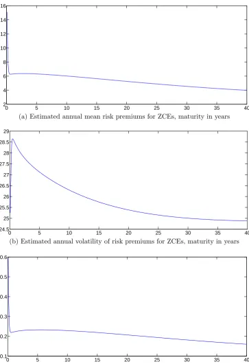
Risk premiums of zero-coupon equities

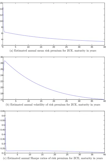
In this section, we look at the equity term structure from another per-spective. In particular, we look at the risk premiums of zero-coupon equities, that is, the one-period return of these assets in excess of the risk-free rate. The reason we look at these quantities is because Lettau and Wachter (2007) use them as empirical support for the value pre-mium. Their rationale is that if we think of value stocks as short-horizon equities since their cash flows are weighted more towards the present, and think of growth stocks as long-horizon equities since their cash flows are weighted more towards the future, then we can only observe the value premium if we see that zero-coupon equities of shorter maturities have higher premiums than zero-coupon equities with longer maturities. Value premium implies a downward sloping equity term structure.

equity is calculated using the following equation:

Rd_n,t+1−Rf =

Pd

n−1,t+1

Pd

nt

−Rf. (1.32)

0 5 10 15 20 25 30 35 40 2

4 6 8 10 12 14 16

Estimated annual mean risk premium for zce, maturity in years

(a) Estimated annual mean risk premium for ZCE, maturity in years

0 5 10 15 20 25 30 35 40

16 18 20 22 24 26 28 30

Estimated annual vol for zce, maturity in years

(b) Estimated annual volatility of risk premium for ZCE, maturity in years

0 5 10 15 20 25 30 35 40

0.2 0.25 0.3 0.35 0.4 0.45 0.5 0.55 0.6 0.65

Estimated annual Sharpe ratio for zce, maturity in years

(c) Estimated annual Sharpe ratios of risk premium for ZCE, maturity in years

Figure 1.7: Estimated risk premiums of zero-coupon equities, equity term structure

1.5

Conclusion

Estimating a Unified Framework of

Co-Pricing Stocks and Bonds

2.1

Abstract

This chapter estimates a maximal identifiable affine term structure model that explains the joint prices of stocks and bonds. Using the test assets of Treasury bonds and dividend strips, it is shown that the estimated model can generally match the time series and cross-sectional proper-ties of zero-coupon bonds, zero-coupon equiproper-ties and the aggregate stock index. Moreover, imposing restrictions prevalent in the co-pricing lit-erature on the maximal model enhances certain features of the model such as the high return of the short-term dividend strip, but reduces the model’s ability to fit other aspects of the data such as the level of the market risk premium.

2.2

Introduction

(1996), Dai and Singleton (2000) and Ang and Piazzesi (2003). However, if investors have access to both stocks and bonds, then the assumption of no-arbitrage will imply cross-market restrictions on the pricing kernel or the stochastic discount factor, which can be used to price all assets in the market. Hence there should exist a unified framework that is able to price both stocks and bonds.

There is now a small and growing literature that tries to use the no-arbitrage affine framework to jointly price stocks and bonds, although each paper has its own focus. In Lettau and Wachter (2011), the focus is on matching an upward sloping bond yield curve and a downward sloping equity yield curve. Koijen, Lustig and Van Nieuwerburgh (2013) is a reduced-form model that uses a cyclical factor to price the book-to-market sorted stock portfolios and maturity sorted bond portfolios. Ang and Ulrich (2012) decomposes expected equity returns into various yields and risk premiums. The key advantage that these affine models have in common is tractability: both stock yields and bond yields are affine functions of the state vector, and the loadings on the state vector are functions of the model parameters. Hence we can easily see how the state vector affects yields analytically.

these models are generally not identified without imposing restrictions. To impose the minimum number of restrictions on the state process such that the model is identified, we can follow Joslin, Singleton and Zhu (2011) (JSZ) to normalize all the models to a canonical form, in which the state vector Xt is entirely latent. As a result of this normalization,

given the same set of asset prices, there is only one model in the canonical form that can generate this set of asset prices. And all the state vectors in the models that can generate this set of asset prices are just rotations (affine transformations) of Xt. Therefore, if we denote the state vector

in the existing papers of co-pricing stocks and bonds as Zt, then the

rotation between Zt and Xt and the minimum number of restrictions on

the process of Xt imply that the process of Zt will also face parameter

restrictions. As the existing models of co-pricing stocks and bonds are usually calibrated and fail to take into account these restrictions in the calibration, this could lead to some of the model parameters being over-restricted (in the sense that the canonical form implies these parameters should be freely estimated but they are instead restricted to zeros or ones) or not identified (in the sense that the canonical form implies these parameters should be restricted to zeros or ones but instead they are freely estimated), which may cause spurious predictions of asset pricing moments.

this paper also utilizes zero-coupon equities in the estimation.

I estimate the model following Joslin, Singleton and Zhu (2011). I first normalize the general model to the canonical form. Then I show that the canonical form is observationally equivalent to another model, in which the N × 1 state vector includes dividend growth and N −1 principal components (PCs) extracted from the yields of zero-coupon bonds and the yields of zero-coupon equities, which can be seen as portfolios of these yields. Including dividend growth in the state vector is motivated by the fact that dividend growth cannot be spanned by the PCs of yields: it can be shown that, when dividend growth is regressed on a constant and the

N−1 PCs of yields, the R-squared is very low, i.e. variation in dividend growth cannot be explained by the PCs of yields. If we do not include dividend growth as a state factor, as the pricing function of zero-coupon equities requires dividend growth to be expressed as an affine function of the state vector we would implicitly assume dividend growth is an affine function of the PCs of yields, which is not the case in the data. Therefore, we must include dividend growth explicitly in the state vector.

for both stocks and bonds well. Moreover, the estimation results show that it is important to take into account the above restrictions to match all the asset pricing moments. It will be seen later that imposing ad-ditional restrictions on top of the identifying restrictions implied by the maximal identifiable model would strengthen some asset pricing features. However, this is achieved at the expense of not matching the other asset pricing features.

By estimating a model of co-pricing stocks and bonds, this paper fills the gap in the literature in which bonds and stocks are usually priced separately. Moreover, in the estimation, I use a maximal identifiable model to make sure I do not impose additional restrictions on the model that may lead to spurious results. Chernov and Mueller (2012) also estimate a model for the bond market, guided by the maximal identifiable model derived from Joslin (2006). Regarding data, I use the dataset on dividend strips provided in van Binsbergen, Brandt and Koijen (2012) to empirically estimate zero-coupon equities, a concept defined as, for example, in Lettau and Wachter (2007) but data on it was missing in the literature. Bekaert and Grenadier (2001) estimate an affine model of co-pricing stocks and bonds as well, but they use only data on the aggregate market index, without using the prices of zero-coupon equities.

2.3

Model and estimation

I assume the economy in this chapter is driven by a latent state vector

Xt, which follows a VAR(1) process under both the physical measure P

and the risk-neutral measure _Q:

∆Xt=K0PX +K1PXXt−1+ ΣXPt,

∆Xt=K0QX +K Q

1XXt−1+ ΣXQt,

whereXtis anN×1 vector,K0PX and K0QX areN×1 vectors,K1PX,K1QX

and ΣX are N ×N matrices and bothPt+1 and Qt+1 are N ×1 vectors of

independent shocks with mean zero and unit variance.

I also assume the short rate and the dividend growth are driven by

Xt, as follows:

rt =ρ0X +ρ01XXt,

where ρ0X is a scalar and ρ1X is an N ×1 vector.

The level of the aggregate dividend of the economy is denoted by Dt.

Letdt= logDt, and the log dividend growth rate from timet−1 to time

t is defined as

∆dt= log

Dt

Dt−1

=δ0X +δ01XXt,

where δ0X is a scalar and δ1X is an N ×1 vector.

Given the above equations, we can derive the prices of zero-coupon bonds, zero-coupon equities and the aggregate market index as shown in Chapter 1. To estimate the asset prices, I use the result of observational equivalence between the latent state vector Xt and a set of observable

state factorsPtas shown in JSZ. The same method was used in Chapter 1

here. Specifically, Pt consists of portfolios of yields PCt and dividend

growth, i.e.

Pt = 

 

PCt

∆dt 

 .

PCt denotes the principal components of bond and equity yields

(port-folio of yields) and is a (N −1)×1 vector. More specifically,

PCt =W yt.

Here yt is a J ×1 vector and includes all the bond and equity yields at

time t. W is (N −1)×J and is the weight of the portfolios. Therefore, given that yt is affine in Xt,

yt=AX +BX0 Xt,

where AX is J×1 and BX is N ×J, Pt is also affine in Xt as

Pt = 

 

PCt

∆dt   =   

W AX

δ0X   +   

W B_X0 δ₁0_X





Xt =A+BXt.

Given the affine relationship between Pt and Xt, we can show that

the economy can be observationally equivalently defined in terms of Pt

as follows:

∆Pt=K0PP +K1PP Pt−1+ ΣPP_t,

∆Pt=K0PQ +K1PQ Pt−1+ ΣPQt,

rt=ρ0P +ρ01PPt,

∆dt=δ0P+δ1P0 Pt.

state process can be estimated by an unrestricted VAR. Then, taking the estimated parameters from the VAR as given, the rest of the parameters are then estimated using MLE.

2.3.1

Data

This section describes the data used in the estimation, including bond yields and the principal components extracted from both zero-coupon bond yields and zero-coupon equity yields. The data on equity yields and dividend growth used in this chapter is the same as in Chapter 1. Previously, there was no empirical counterpart for zero-coupon equities, so in the literature the estimation of the co-pricing model, e.g. in Bekaert and Grenadier (2001), can only use the aggregate equity price, which is the sum of the prices of zero-coupon equities of all maturities. Hence, the information on the term structure of equities was missing in the estimation. However, Chapter 1 shows that, using dividend strip prices, the S&P 500 index and the dividend series provided by van Binsbergen, Brandt and Koijen (2012), we can construct “equity yields” that are comparable to “bond yields”.

Bond yields

slop-ing. Standard deviations of bond yields generally decrease with maturity. Finally, yields are highly autocorrelated, with increasing autocorrelation at longer maturities. In dealing with the stationarity of bond yields at various maturities, I follow the same reasoning as in Chapter 1 for the bond yield of one-month maturity. That is, I assume all bond yields are stationary, but allow them to have a very low speed of mean reversion.

19960 1998 2000 2002 2004 2006 2008 2010 1

2 3 4 5 6 7

CMT data, zcb yields, annual percentages, 1996m2:2009m10

1m 6m 1yr 2yr 3yr 5yr 7yr 10yr

Figure 2.1: Zero-coupon bond yields, 1996m2:2009m10

Table 2.1: Summary statistics of the U.S. bond yields (all numbers are in annualized percentages)

Maturity (years) 1m 6m 1y 2y 3y 5y 7y 10y Panel A: Data

Mean 3.37 3.57 3.69 3.95 4.13 4.45 4.71 4.87 Standard deviation 1.87 1.90 1.84 1.74 1.60 1.33 1.19 1.02

Co-pricing factors

happen to use six state factors to drive their economy. If a six-factor state vector is also employed here, then the state vector in any of the papers mentioned above can be viewed as a rotation of the state vector in this chapter. Hence it is easier to translate between each paper’s re-sults. More importantly, whereas existing papers on co-pricing set many additional restrictions on top of the minimal set of restrictions imposed by the maximal identifiable model, we can impose the same set of re-strictions on the estimated maximal identifiable model in this chapter, and see how these additional restrictions affect asset pricing moments. Hence, five PCs are chosen and, together with monthly dividend growth for the same sample period taken from van Binsbergen, Brandt and Koi-jen (2012), they make up the six state factors that drive the economy and all asset prices.

2.3.2

Estimation results

This subsection shows the estimation results and compares the data with the model-implied asset pricing moments of coupon bonds, zero-coupon equities, dividend strips and the aggregate stock market index.

Model parameters

(λQ_{, r}Q

∞, ΣP, δ0X, δ1X) are estimated in MLE and their estimates are

shown in Table 2.2 and Table 2.3. From the estimates of (λQ

i +1)s, we can

see that the estimated state process has real and distinct eigenvalues, and because all (ˆλQ

i +1)s are between zero and one the estimated state process

the OLS estimates ofKP

0P andK1PP +I. Estimates are in annual numbers

and their standard deviations are provided in parentheses.

Table 2.2: Maximum likelihood estimates of the risk-neutral parameters, unrestricted co-pricing model

λQ

1+1 λQ2+1 λQ3+1 λ4Q+1 λQ5+1 λQ6+1 r∞Q

Estimate 0.9967 0.9930 0.9358 0.2799 0.2779 0.2761 6.6794 Standard (0.0010) (0.0007) (0.0031) (0.0019) (3.6189e-5) (0.0017) (0.5841) deviation

δ0X δ1X,1 δ1X,2 δ1X,3 δ1X,4 δ1X,5 δ1X,6

Estimate 0.0185 −0.0019 0.7058 0.4636 −0.5838 0.0083 0.5380 Standard (0.0118) (1.6274e-5) (0.0012) (0.0089) (0.0013) (0.0001) (0.0047) deviation

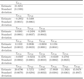
Table 2.3: Maximum likelihood estimates of the conditional covariance, unrestricted co-pricing model

ΣP,11

Estimate 21.0251 Standard (0.1593) deviation

ΣP,21 ΣP,22

Estimate −0.2952 0.5408 Standard (0.0015) (0.0061) deviation

ΣP,31 ΣP,32 ΣP,33

Estimate 0.0383 −0.2494 0.2995 Standard (0.0001) (0.0037) (0.0043) deviation

ΣP,41 ΣP,42 ΣP,43 ΣP,44

Estimate 0.1310 0.0836 −0.0658 0.1194 Standard (0.0012) (0.0023) (0.0001) (0.0041) deviation

ΣP,51 ΣP,52 ΣP,53 ΣP,54 ΣP,55

Estimate −0.0507 −0.0234 0.1276 −0.0239 0.2783 Standard (0.0002) (0.0001) (0.0010) (0.0002) (0.0025) deviation

ΣP,61 ΣP,62 ΣP,63 ΣP,64 ΣP,65 ΣP,66

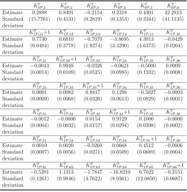
Table 2.4: Maximum likelihood estimates of the physical parameters, unrestricted co-pricing model

KP

0P,1 K0PP ,2 K0PP ,3 K0PP ,4 K0PP ,5 K0PP ,6

Estimate 0.2898 0.8491 −0.2154 0.2318 0.4301 42.2813 Standard (15.7761) (0.4531) (0.2819) (0.1353) (0.2344) (41.1135) deviation

KP

1P,11+1 K1PP ,12 K1PP ,13 K1PP ,14 K1PP ,15 K1PP ,16

Estimate 0.7730 0.6810 −0.7070 −3.8695 4.3913 −0.0429 Standard (0.0484) (0.3778) (1.8274) (3.4290) (4.6373) (0.0264) deviation

KP

1P,21 K1PP ,22+1 K1PP ,23 K1PP ,24 K1PP ,25 K1PP ,26

Estimate −0.0043 0.9948 −0.0326 −0.0621 −0.5000 0.0009 Standard (0.0014) (0.0109) (0.0525) (0.0985) (0.1332) (0.0008) deviation

KP

1P,31 K1PP ,32 K1PP ,33+1 K1PP ,34 K1PP ,35 K1PP ,36

Estimate 0.0001 0.0082 0.8817 0.1298 −0.5027 −0.0003 Standard (0.0009) (0.0068) (0.0326) (0.0613) (0.0829) (0.0005) deviation

KP

1P,41 K1PP ,42 K1PP ,43 K1PP ,44+1 K1PP ,45 K1PP ,46

Estimate −0.0012 −0.0006 0.0154 0.9129 0.1006 −0.0000 Standard (0.0004) (0.0032) (0.0157) (0.0294) (0.0398) (0.0002) deviation

KP

1P,51 K1PP ,52 K1PP ,53 K1PP ,54 K1PP ,55+1 K1PP ,56

Estimate 0.0010 0.0020 −0.0260 0.0668 0.4512 −0.0006 Standard (0.0007) (0.0056) (0.0271) (0.0509) (0.0689) (0.0004) deviation

KP

1P,61 K1PP ,62 K1PP ,63 K1PP ,64 K1PP ,65 K1PP ,66+1

Estimate −0.5201 1.1313 −1.7847 −16.8210 6.7022 −0.2151 Standard (0.1261) (0.9846) (4.7622) (8.9361) (12.0850) (0.0687) deviation

Equities

a. Equity yields

Table 2.5: Estimation results: moments comparison for equity yields, annual percentages, unrestricted co-pricing model

Maturity 6m 12m 18m 24m 50y Panel A: Data

Mean 6.91 4.38 3.53 3.11 1.85 Standard deviation 28.60 14.17 9.36 6.96 0.38

Panel B: Model

Mean 6.94 4.33 3.50 3.11 1.89 Standard deviation 28.65 14.13 9.30 6.90 0.38

b. Return of the dividend strip and the aggregate market

Just as in Chapter 1, we calculate the return of the dividend strip of short maturity and the return of the aggregate market to see whether the slope of the equity term structure is downward sloping or upward sloping. However, in this chapter, the slope of the equity term structure is backed out from the joint estimation of both the bond yield curve and the equity yield curve. Hence it is interesting to see that, after adding bond data, the model-implied slope of the equity term structure can still maintain its downward slope given an upward sloping bond yield curve. Table 2.6 repeats for convenience Table 1.5 in Chapter 1, which shows the return of the short-term dividend strip of average maturity between 1.3 years and 1.9 years, the return of the S&P 500 index and their returns in excess of the short rate.

Table 2.6: Data: summary statistics of the return of the short-term strip and the market

R_{short strip} R_{short strip}−Rf R_market R_market−Rf

Mean 13.90 10.53 6.67 3.29

Standard 27.03 27.04 16.26 16.22

deviation

Sharpe ratio 0.39 — 0.20 —

calcu-lated using the equations below:

Rs_t+1 = P

s

n−1,t+1+Dt+1

Ps

n,t

−1,

where Ps

n,t = Pn

i=1P d

i,t is the time-t price of the dividend strip of

matu-rity n, the sum of the prices of the zero-coupon equities from maturity 1 to n;

Rm_t+1 = P

m

t+1+Dt+1

Pm

t

−1,

where P_tm = P∞ i=1P

d

i,t is the time-t market index, the sum of prices of

zero-coupon equities from maturity 1 to ∞.

Table 2.7 and Table 2.8 show that the model-implied equity term structure is downward sloping, just as observed in the data. The returns and excess returns of the short-term dividend strips of maturities of fif-teen months to twenty-three months are slightly lower than the returns of the short-term dividend strip, but they are comparable. Moreover the market return and excess market return are both closely matched. Table 2.7: Summary statistics of the return of the short-term strip and the market, unrestricted co-pricing model

R15m R16m R17m R18m R19m R20m R21m R22m R23m R_market Mean 11.90 11.76 11.64 11.54 11.44 11.36 11.28 11.21 11.15 7.05 Standard 26.48 26.57 26.65 26.72 26.78 26.84 26.89 26.93 26.97 24.72 deviation

Sharpe 0.32 0.32 0.31 0.31 0.30 0.30 0.29 0.29 0.29 0.15 ratio

Table 2.8: Summary statistics of the excess return of the short-term strip and the market, unrestricted co-pricing model

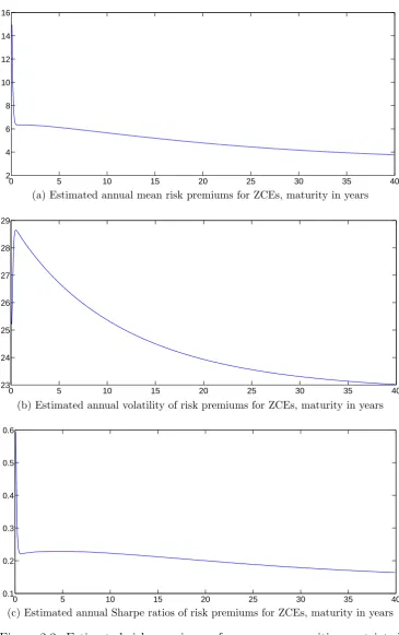
c. Risk premiums of zero-coupon equities

Using

Rd_n,t+1−Rf =

P_nd_−1,t+1 Pd

nt

−Rf

0 5 10 15 20 25 30 35 40 2

4 6 8 10 12 14 16

Estimated annual mean risk premium for zce, maturity in years

(a) Estimated annual mean risk premiums for ZCEs, maturity in years

0 5 10 15 20 25 30 35 40

24.5 25 25.5 26 26.5 27 27.5 28 28.5 29

Estimated annual vol for zce, maturity in years

(b) Estimated annual volatility of risk premiums for ZCEs, maturity in years

0 5 10 15 20 25 30 35 40

0.1 0.2 0.3 0.4 0.5 0.6

Estimated annual Sharpe ratio for zce, maturity in years

(c) Estimated annual Sharpe ratios of risk premium for ZCEs, maturity in years

Bond yields

The estimation results regarding bonds are shown in Table 2.9. The table shows that model-implied bond yields exhibit the same characteristics as the observed yields, i.e. bond yields means are almost monotonically increasing with maturity, while the standard deviations of bond yields are generally decreasing in maturity. The close match in magnitudes of both the means and the standard deviations between the estimated and the observed bond yields shows that the co-pricing framework can match bond yields well. Hence this shows that the co-pricing framework in this paper can generate both the downward sloping equity yield curve and the upward sloping bond yield curve.

Table 2.9: Estimation results: moments comparison for zero-coupon bonds (all numbers are in annualized percentage), unrestricted co-pricing model

Maturity 1m 6m 1y 2y 3y 5y 7y 10y Panel A: Data

Mean 3.37 3.57 3.69 3.95 4.13 4.45 4.71 4.87 Standard deviation 1.87 1.90 1.84 1.74 1.60 1.33 1.19 1.02

Panel B: Model

Mean 3.36 3.59 3.70 3.93 4.12 4.43 4.67 4.94 Standard deviation 1.84 1.98 1.86 1.67 1.54 1.35 1.21 1.04

2.4

Restricted Model

2.4.1

Comparison with Lettau and Wachter (2011)

This section illustrates the importance of taking into account the re-strictions implied by the maximal identifiable model. I will use Lettau and Wachter (2011), one of the existing papers of co-pricing stocks and bonds, as an example to show that it is important to take into account the restrictions in order to match all the asset pricing moments.

The model in this paper and the model in Lettau and Wachter (2011) are both designed to price bonds and equities and, in particular, to simul-taneously generate an upward sloping bond yield curve and a downward sloping equity yield curve. Both papers belong to the same class of mod-els, i.e. Gaussian affine term structure modmod-els, and have the same num-ber of factors. Hence, once they are normalized to the same canonical form, the resulting two models should have very similar state processes. However, in Lettau and Wachter (2011), the model is calibrated rather than estimated and they implicitly impose additional restrictions on their canonical form. For example, in their model, one of the assumptions is that only dividend risk is priced directly and hence the price of risk ma-trix reduces to a single time varying vector and the time variation in risk premiums depends only on a one-dimensional state variable. Hence it will be interesting to see how this restriction affects asset-pricing predictions. The estimation results of the restricted model are shown below.

2.4.2

Estimation results

Model parameters

Table 2.10, Table 2.11 and Table 2.12 list the estimates of the model parameters. From the estimates of the (λQ

i + 1)s, we can see that the

restricted state process is also stationary under _Q.

Table 2.10: Maximum likelihood estimates of the risk-neutral parameters, restricted co-pricing model

λQ

1+1 λQ2+1 λQ3+1 λ4Q+1 λQ5+1 λQ6+1 r∞Q

Estimate 0.9951 0.9919 0.9496 0.2793 0.2772 0.2753 6.2736 Standard (0.0015) (0.0148) (0.0324) (0.0076) (0.0001) (0.0065) (7.1347) deviation

δ0X δ1X,1 δ1X,2 δ1X,3 δ1X,4 δ1X,5 δ1X,6

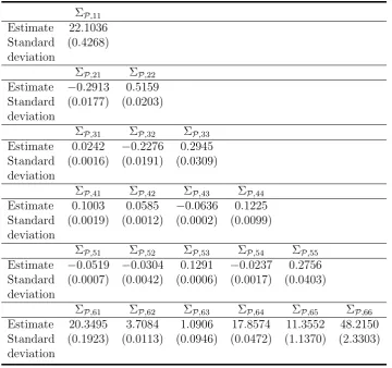
Table 2.11: Maximum likelihood estimates of the conditional covariance, restricted co-pricing model

ΣP,11

Estimate 22.1036 Standard (0.4268) deviation

ΣP,21 ΣP,22

Estimate −0.2913 0.5159 Standard (0.0177) (0.0203) deviation

ΣP,31 ΣP,32 ΣP,33

Estimate 0.0242 −0.2276 0.2945 Standard (0.0016) (0.0191) (0.0309) deviation

ΣP,41 ΣP,42 ΣP,43 ΣP,44

Estimate 0.1003 0.0585 −0.0636 0.1225 Standard (0.0019) (0.0012) (0.0002) (0.0099) deviation

ΣP,51 ΣP,52 ΣP,53 ΣP,54 ΣP,55

Estimate −0.0519 −0.0304 0.1291 −0.0237 0.2756 Standard (0.0007) (0.0042) (0.0006) (0.0017) (0.0403) deviation

ΣP,61 ΣP,62 ΣP,63 ΣP,64 ΣP,65 ΣP,66

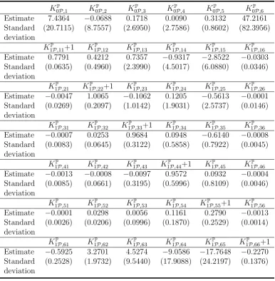
Table 2.12: Maximum likelihood estimates of the physical parameters, restricted co-pricing model

KP

0P,1 K0PP ,2 K0PP ,3 K0PP ,4 K0PP ,5 K0PP ,6

Estimate 7.4364 −0.0688 0.1718 0.0090 0.3132 47.2161 Standard (20.7115) (8.7557) (2.6950) (2.7586) (0.8602) (82.3956) deviation

KP

1P,11+1 K1PP ,12 K1PP ,13 K1PP ,14 K1PP ,15 K1PP ,16

Estimate 0.7791 0.4212 0.7357 −0.9317 −2.8522 −0.0303 Standard (0.0635) (0.4960) (2.3990) (4.5017) (6.0880) (0.0346) deviation

KP

1P,21 K1PP ,22+1 K1PP ,23 K1PP ,24 K1PP ,25 K1PP ,26

Estimate −0.0047 1.0065 −0.1062 0.1205 −0.5613 −0.0001 St