A Novel Blind SR Method to Improve the Spatial Resolution of Real Life Video Sequences

© 2017, IRJET | Impact Factor value: 5.181 | ISO 9001:2008 Certified Journal

| Page 1577

A Novel Blind SR Method to Improve the Spatial Resolution of Real Life

Video Sequences

1

_{W. RAJESH KUMAR,}

_{U. SATHISH KUMAR}

(M.Tech.)

_,

_{Dept of CSE, Acharya Nagarjuna University, Guntur, AP, (522510), INDIA}

Assistant Professor

_{,(,M.Tech,(Ph.d)),}

_{Dept of CSE, Acharya Nagarjuna University, Guntur, AP, (522510), INDIA}

---***---

Abstract-

Keywords: Video super resolution, blur deconvolution, blind estimation, Huber Markov random field (HMRF).

1. INTRODUCTION:

Multi-frame super resolution, namely estimating the higher frames from a low-res sequence, is one of the fundamental problems in computer vision and has been extensively studied for decades. The problem becomes particularly interesting as high-definition devices such as high definition television HDTV (1920 × 1080) dominate the market. The resolution of various display has increased dramatically recently, including the New iPad (2048 × 1536), 2012 Macbook Pro (2880 × 1800), and ultra high definition television UHDTV (3840 × 2048 or 4K, 7680 × 4320 or 8k). As a result, there is a great need for converting low resolution, low-quality videos into

high-resolution, noise free videos that can be pleasantly viewed on these high resolution devices.

Although a lot of progress has been made in the past 30 years, super resolving real-world video sequences still remains an open problem. Most of the previous work assumes that the underlying motion has a simple parametric form, and/or that the blur kernel and noise levels are known. But in reality, the motion of objects and cameras can be arbitrary, the video may be contaminated with noise of unknown level, and motion blur and point spread functions can lead to an unknown blur kernel. Therefore, a practical super resolution system should simultaneously estimate optical flow [3], noise level [7] and blur kernel [4] in addition to reconstructing the higher image. As each of these problems has been well studied in computer vision, it is natural to combine all these components in a single framework without making simplified assumptions.

In this paper, we propose a Bayesian framework for adaptive video super resolution that incorporates high-resolution image reconstruction, optical flow, noise level and blur kernel estimation. Using sparsity prior for the high-res image, flow fields and blur kernel, we show that super resolution computation is reduced to each component problem when other factors are known, and the MAP inference iterates between optical flow, noise estimation, blur estimation and image reconstruction. As shown in Figure 1 and later examples, our system produces promising results on challenging real-world sequences despite various noise levels and blur kernels, accurately reconstructing both major structures and fine texture details. In-depth experiments demonstrate that our system outperforms the state-of-the-art super resolution systems [1], [8], [9] on challenging real-world sequences.

2. LITERATURE SURVEY

© 2017, IRJET | Impact Factor value: 5.181 | ISO 9001:2008 Certified Journal

| Page 1578

model global translational scene motion, and take advantage of the sampling theory to enable effect restoration made possible by the availability of multiple observation images. It is interesting to note that the methods we discuss here include the earliest investigation of the super-resolution problem, and although there are significant disadvantages in the frequency domain formulation, work has continued in this area until relatively recently when spatial domain techniques, with their increased flexibility, have become more prominent. This does not however mean to say that frequency domain techniques be ignored. Indeed, under the assumption of global translational motion, frequency domain methods are computationally highly attractive. We begin our review of frequency domain methods with the seminal work of Tsai and Huang [4].

In this paper [3], the author describes Printing from an NTSC source and conversion of NTSC source material to high-definition television (HDTV) format are some of the recent applications that motivate super resolution (SR) image and video reconstruction from lower resolution (LR) and possibly blurred sources. Existing methods for SR image reconstruction are limited by the assumptions that the input LR images are sampled progressively, and that the aperture time of the camera is zero, thus ignoring the motion blur occurring during the aperture time. Because of the observed adverse effects of these assumptions for many common video sources, this paper proposes i) a complete model of video acquisition with an arbitrary input sampling lattice and a nonzero aperture time, and ii) an algorithm based on this model using the theory of projections onto convex sets to reconstruct SR still images or video from an LR time sequence of images.

Kim et al [45] in their paper, propose a recursive algorithm for restoration of super resolution images from noisy and blurred observations. They use the aliasing relationship between the under sampled frames and the reference image, to develop a weighted recursive least-squares theory based algorithm in the wave number domain. This algorithm is efficient because interpolation and noise removal are performed recursively and in addition, it is highly suitable for implementation through the massively parallel computational architectures currently available. Accurate knowledge of the relative scene locations sensed by each pixel in the observed images is necessary for super resolution. This information is available in image regions where local deformation can be described by some parametric function. Such functions can describe, for example, perspective transformation. Authors assumed that local motion can be described by translations and

rotations only, but the approach is applicable also for other image motion models.

3. PROPOSED METHOD

A. Observation Model

Fig 1: Estimation of fk frame from LR video sequences

As shown in Fig. 1, a sliding window (temporal) of length M + N + 1 (with M frames backward and N frames

forward) is overlaid around each LR frame gk of size

, and all LR frames inside the window are

combined through the SR process to generate the HR

reference frame fk of size . Here, Nxand Ny are

frame dimensions in two spatial directions and C is the number of color channels. The linear forward imaging model that illustrates the process of generating a LR frame

gi inside the window from the HR frame fk is given by:

( ) [ ( ( )) ( )] ( )

( )

where P is the total number of frames, (x↓, y↓) and (x, y) indicate the pixel coordinates in LR and HR image planes respectively, L is the down sampling factor or SR up scaling

ratio (so that , and is the

two-dimensional convolution operator. According to this

model, the HR frame fk is warped with the warping

function mk,i , blurred by the overall system PSF h, down sampled by factor L, and finally corrupted by the additive noise nk,i . It is more convenient to express this linear process in the vector-matrix notion:

gi = DHMk,ifk + ni---(2)

© 2017, IRJET | Impact Factor value: 5.181 | ISO 9001:2008 Certified Journal

| Page 1579

indicating a vector of size , matrices Mk,i and H

are the motion (warping) and convolution operators of

size , , D is the down sampling matrix of

size , and gi and ni are vectors of the ith

LR frame and noise respectively, both of size .

The matrix Mk,i registers (or motion compensates) the

reference frame fk to match the frame fi . As a result, Mkk is an identity (unit) matrix since no motion compensation is required between a HR frame and its coincident LR frame. For a blur deconvolution (BD) problem (i.e. L = 1), D is the identity matrix and so the input and output videos are of the same size. Hence BD can be considered as a special case of SR. The objective in SR and BD is to estimate the HR

frames fk and the blur H given the LR frames gi while the

motion Mk,i and the noise ni are unknown as well.

B. Color Space

The human visual system (HVS) is less sensitive to chrominance (color) than to luminance (light intensity). In the RGB (red, green, blue) color space, the three color components have equal importance and so all are usually stored or processed at the same resolution. But a more efficient way to take the HVS perception into account is by separating the luminance from the color information and representing luma with higher resolution than chroma.

A popular way to achieve this separation is to use the YCbCr color space where Y is the luma component (computed as a weighted average of R, G, and B) and Cb and Cr are the blue-difference and red-difference chroma components. The YUV video format is commonly used by video processing algorithms to describe video sequences encoded using YCbCr.

In our implementation, video sequences can be processed in either RGB or YUV formats. In the former case, SR is used to increase the resolution of all R, G, and B channels. However in the latter one, only the Y channel is processed by SR for faster computation while the Cb and Cr channels are simply up scaled to the resolution of the super-resolved Y channel using a single-frame up sampling method such as bilinear or bi cubic interpolation. The obtained results related to these two cases are comparable using a subjective quality assessment.

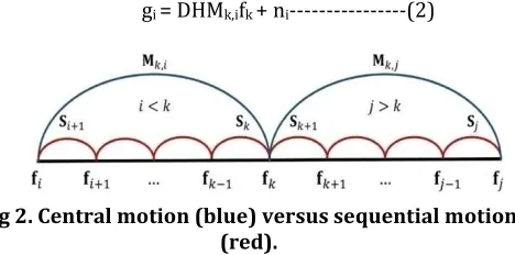
C. Motion Estimation

Accurate motion estimation (registration) with sub pixel precision is crucial for video SR to achieve a good performance. Two different approaches can be considered

for registration in video SR: central and sequential (Fig. 2). In the former, motion is directly computed between each reference frame and all LR frames inside its sliding window (Fig. 1). By contrast, in the latter, each frame is registered against its previous frame; then to use with SR, sequential motion fields must be converted to central fields for registration as follows: if Si = [ Sxi, Syi ] is the

sequential motion field for the ith _{frame (w.r.t. the (i −1)th}

frame), then Mk,i = [ Mxk,i , Myk,i ] , the central motion field

for the ith frame when the central frame is the kth _{frame is}

obtained as:

∑

∑

( )

Where I is the identity matrix.

With the sequential approach in SR, each frame needs to be registered only against the previous frame, whereas with the central approach each frame is registered against all neighboring frames within its reconstruction window. Therefore, the computational complexity and the storage size of the motion fields in the central approach is higher than that of using the sequential approach.

D. B LUR ESTIMATION

In a multi-channel BD problem, the blurs could be estimated accurately along with the HR images [27]. However in a blind SR problem with a possibly different blur for each frame, some ambiguity in the blur estimation is inevitable due to the downsampling operation [19]. By contrast, in a blind SR problem in which all blurs are supposed to be identical or have gradual changes over time, such an ambiguity can be avoided the assumption of identical (or gradually changing) blurs makes it possible to separate the registration and upsampling procedures from the deblurring process which significantly decreases the blur estimation complexity.

© 2017, IRJET | Impact Factor value: 5.181 | ISO 9001:2008 Certified Journal

| Page 1580

Section III-D.

E. Frame up sampling:

In [2] we discuss the situations in which the warping and blurring operations in (2) are commutable. Although for videos with arbitrary local motions this commutability does not hold exactly for all pixels, however we assume here that this is approximately satisfied. The ultimate appropriateness of the approximation is validated by the eventual performance of the algorithm that is derived based on this model. With this assumption, (2) can be rewritten as:

( )

Where = is the upsampled but still blurry frame.

Equation (4) suggests that we can first construct the upsampled frames zk using an appropriate fusion method

and then apply a deblurring method to to estimate

and h.

If noise characteristics are also the same for all frames, an

appropriate way to estimate is using the NUI method

[3]–[5]. In NUI, the pixels of all LR frames are projected on to the HR image grid according to their motion fields, and then the intensities of the true locations on the grid are computed via interpolation [2].

E. FRAME DEBLURRING:

After upsampling the frames, we use the following cost function, J, to estimate the HR frames fk having an estimate of the blur h (or H):

( ) ‖ ( )‖ ∑‖ ( )‖ ( )

where · 1 denotes the l1 norm (defined for a sample vector x with elements xi as x = i | xi| ), λn is the regularization coefficient, ρ(·) is the vector Huber function,

ρ(·) 1 is called the Huber norm, and ∇ j (i = 1,. . ., 4) are the

gradient operators in 0°, 45°, 90° and 135° spatial directions [2]. The first term in (5) is called the fidelity term which is the Hubernorm of error between the observed and simulated LR frames. While in most works the l2-norm is used for the fidelity term, we use the robust Huber norm to better suppress the outliers resulting from inaccurate registration. The next two terms in (5) are the regularization terms which apply spatiotemporal

smoothness to the HR video frames while preserving the edges.

Each element of the vector function ρ(·) is the Huber function defined as:

( ) { | |

| | | | ( )

The Huber function ρ(x) is a convex function that has a quadratic form for values less than or equal to a threshold T and a linear growth for values greater than T. The Gibbs PDF of the Huber function is heavier in the tails than a Gaussian. Consequently, edges in the frames are less penalized with this prior than with a Gaussian (quadratic) prior.

To minimize the cost function in (5), we use the conjugate gradient (CG) iterative method [30] because of its simplicity and efficiency. Compared to some other iterative methods such as Gauss-Seidel (GS) or SOR that need explicit derivation of matrix A when solving a linear equation Ax = b, CG can decompose the matrix A to concatenation of filtering and weighting operations. However, CG can only be used with linear equation sets, whereas the cost function in (5) is non quadratic and so its derivative is nonlinear. To overcome this limitation, we use lagged diffusivity fixed-point (FP) iterative method [31] to lag the diffusive term by one iteration [15]. Using this method for a sample vector x, at the nth iteration the non-quadratic Huber-norm ρ(xn)1 is replaced by the following quadratic form:

‖ ( )‖ ( ) ( ) ‖ ‖ ( )

Where Vn is the following diagonal matrix:

({

_⁄ ) (

In (8) the dots above the division and comparison operators indicate element-wise operations. Applying the FP method to (5) and setting the derivative of the cost function with respect to fk to zero results in the following linear equation set:

_∑

_{( )}

© 2017, IRJET | Impact Factor value: 5.181 | ISO 9001:2008 Certified Journal

| Page 1581

( ( ₎₎

( ( _{)) (}

We discuss how to update the regularization parameter λn at each iteration in Section III-D.

F. Blur estimation:

Within an image or video frame, non-edge regions and weak structures are not appropriate for blur estimation. Hence, more accurate results would be obtained if the estimation is not performed in such regions. For this reason, in [11] and [33] the user should first manually select a region with rich edge structure, whereas in [2], [13], [14], and [34] the most salient edges are automatically chosen. Moreover, sharpening salient edges would also improve the accuracy of blur estimation. a lowpass Gaussian filtering is utilized before shock filtering. A similar concept for the blur estimation is exploited in [37] in which the image is first sharpened by redistributing the pixels along the edge profiles in such a way that ant aliased step edges are produced. Having the sharpened image and the blurry input image, the blur is then estimated using a maximum a posteriori (MAP) framework.

In our work, we employ the edge-preserving smoothing method of [40] in which the number of surviving edges after smoothing is globally controlled by the regularization coefficient. This feature is helpful when one desires to limit the number of salient edges at each iteration. This smoothing method aims to keep an intended number of non-zero gradients through l0 gradient minimization using the following cost function:

( _{) ‖ ‖ (‖ ‖ ‖ ‖ ) ( )}

where fn k is the output of the edge-preserving smoothing algorithm and the l0 norm is defined as x 0 = # (i| xi = 0). Unlike shock filtering, this smoothing method does not need pre-filtering of noise.

Though sufficient edge pixels are required for accurate blur estimation, it is shown in [14] that structures with scales smaller than the PSF support could harm blur estimation. Inspired by that work, we define Rkn in (12) to measure the usefulness of each pixel for blur estimation:

| | ( )

Where A and B are the convolution operators for the spatial filters a and b, respectively, as defined below:

[ ] ( )

* + (

In (13) and (14), a is the all-ones filter of size 11 × 11 and b is the sum-of-gradients filter. According to (12)-(14), to

compute , the sum of gradient components of

usually has a small value at the location of narrow edges and smooth regions.

𝑓0𝑘 𝑧𝑘

Algorithm 1 Blur Estimation Procedure

Require: 𝑔 𝑔𝑝 𝜆𝑚𝑖𝑛 Υ𝑚𝑖𝑛 and initials 𝑜 𝜆𝑜 𝛾𝑜 𝛽𝑜 𝑇𝑜 𝑇20 Set n: =0 % Am loop iteration number

S: = # of scales

Use luma or one color channel of 𝑔 𝑔𝑝1

for k: =1 to 𝑃 do % Loop on 𝑷𝟏reference frames if L>1 then % For SR reconstruction 𝑧𝑘 𝑁𝑈𝐼(𝑔𝑘 𝑀 𝑔𝑘 𝑁)

else % For BD reconstruction 𝑧𝑘 𝑔𝑘

end if

%HR frame and blur estimation

for s: =1 to S do % Multi-scale approach Rescale 𝑧𝑘 𝑓𝑘𝑛 𝑎𝑛𝑑 𝑛

% AM loop iteration

while “AM stopping criterion “is not satisfied do n=n+1

% Updating procedure for f compute 𝐕𝐧 _{and 𝐖}

𝑗𝑛 using (10) update 𝜆𝑛

while 𝐟𝑛 _{does not satisfy “CG stopping criterion” do} 𝑓𝑘𝑛: = CG iteration for system in (9); starting at

𝑓𝑘𝑛

end while

Apply constraints on 𝑓𝑘𝑛 % Updating procedure for 𝒉𝒏

Update 𝛾𝑛 _𝛽𝑛 _𝑇𝑛 _{𝑎𝑛𝑑 𝑇} 2𝑛 Compute the smoothed frame 𝑓𝑘𝑚 from (11) Compute ∇𝑓𝑘 𝑛 from (15)

Edge tapping of ∇𝑓𝑘 𝑛 Compute 𝑘𝑛(𝑥 𝑦) from (17) Apply constraints on 𝑛 end while

end for end for

is computed first, then at each pixel it is summed up with the values of all neighboring pixels, and finally its absolute value is obtained.

© 2017, IRJET | Impact Factor value: 5.181 | ISO 9001:2008 Certified Journal

| Page 1582

Then is refined by only retaining strong and non-spike

edges:

_{ | |

( )

Where and are threshold parameters which

decrease at each iteration.To avoid ringing artifact, we

apply the MATLAB function edgetaper() to ∇ . Then we

estimate each blur hk using the cost function J(h) below:

( ) ∑‖ ‖ ‖ ‖ ( )

Where P1 ≤ M + N and is the convolution

matrix of fk. Since J(h) in (16) is quadratic, it can be easily minimized by pixel-wise division in the frequency domain [41] as:

( )

_{(∑ ∑ {* (} ̅̅̅̅̅̅̅̅̅̅̅̅̅̅̅̅̅̅̅̅̅_{) ̇ (} ̇ ₎

̇ ( ( ) ̇ ( ̇ ̇ )_{) +} ̇_{[| ( ) ̇ (} ̇ _)| ̇

| ( )| ̇_{]}) ( )}

Where ∇i(i = 1, 2) is ∇x or ∇y, F(·) and F−1(·) are

FFT and inverse-FFT operations, and (·) is the complex conjugate operator. We then apply the following constraints to the estimated PSF: its negative values are set to zero, then the PSF is normalized to the range [0, 1], and centered in its support window.

D. Overall Optimization for Blur Estimation:

The overall optimization procedure for estimating the PSF is shown in Algorithm 1. The HR frames and the PSF are sequentially updated within the AM iterations. We use a multi-scale approach to avoid trapping in local

minima. The regularization coefficients in (9) and in

(17) decrease at each AM (alternating minimization)

iteration up to some minimum values and ,

respectively (see [2] for a discussion). The variation of these coefficients is given by:

(

) ( ) ( )

Where r is a scalar less than 1. Also the values of βn in (11) and Tn 1 and T2n in (15) fall at each AM iteration which increases the number of contributing pixels to blur estimation as the optimization proceeds.

IV. FINAL HR FRAME ESTIMATION

After the PSF estimation is completed, the final HR frames are reconstructed through minimizing the following cost function:

( ) ∑ ( ∑ ‖ ( ( ))‖

∑‖ ( )‖ ( )

)

Where Ok,i is a diagonal weighting matrix that assigns less weights to the outliers. Minimizing this cost function with respect to fk yields:

Algorithm 2 Final Frame Estimation Procedure

Require: 𝑔 𝑔𝑝 and 𝜆

1: Set n: = 0 % FP loop iteration number

2: for k: =1 to P do % Loop on P reference frames

3: Estimate sequential motion fields 𝑆 𝑆𝑝

4:Compute central motion fields 𝑀 𝑀𝑝 using

(??)

5:Estimate the blur h using Algorithm 1

7:% Estimate HR frames using FP loops

8:while ‘’FP stopping criterion” is not satisfied do

9: n=n+1

10: Compute 𝐎𝑘𝑗𝑛 using (22)

11: Compute 𝐕𝑛_{and 𝐖}

𝑗𝑛 using (21) 12: While𝑓𝑛 _{does not satisfy “”CG stopping}

criterion” do

13:𝑓𝑘𝑛 : = CG iteration for system in (20); starting at

𝑓𝑘𝑛

14: end while

15 Apply constraints on 𝑓𝑘𝑛

17: end while

© 2017, IRJET | Impact Factor value: 5.181 | ISO 9001:2008 Certified Journal

| Page 1583

( ∑ ∑

)

( )

where

( ( ))

( ( )) ( )

and the m-th diagonal element of Onk,i is computed according to:

[ ] {

‖ ( ( ))‖

} ( )

Where in (22) Rm is a patch operator which extracts a patch of size q × q centered at the m-th pixel of fk,i .

The final frame estimation procedure is demonstrated in Algorithm 2.

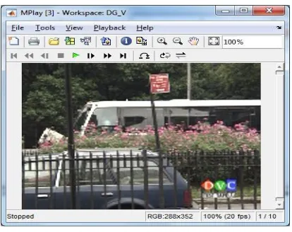
5. Experimental results

In this section, the performance of our method is evaluated and compared with the state-of-the-art video SR methods 3D-ISKR 4 [38] and Fast Upsampler[42] which are available for public evaluation, and also with the commercial software Video Enhancer[43]. Among these three, we only display the results from 3D-ISKR[38]. This non-blind SR method does not include a deblurring step, so we post process its outputs with the deblurring method of [39]. Different parameters for deblurring were tried out in each experiment to get the best possible outcomes from 3D-ISKR. Furthermore, since 3D-ISKR implementation does not estimate pixels near frame boundaries, we remove the boundaries from the reconstructed frame before an objective evaluation.

Fig 1: Proposed method video sequence

Fig 2: degraded video sequence

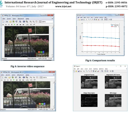
© 2017, IRJET | Impact Factor value: 5.181 | ISO 9001:2008 Certified Journal

| Page 1584

Fig 6: Comparison results

Fig 4: inverse video sequence

Fig 5: Bi cubic interpolation pervious method Fig 7: PSNR values for proposed and pervious method

CONCLUSION:

In this paper by using the blind deconvolution technique the low resolution video is converted into a super resolution form. The main problem in the real-life video sequences is in the nature of motion the frame will become blur. By using the non-uniform interpolation (NUI) SR method the input frames are upsampled and the blur is estimated. In the estimation process an assumption is made as the blur is either identical or have a slow variations over time. After performing upsampling of frames the blur is determined for some enhanced edges. To obtain the final reconstructed frames the previous frames are removed and non-blind iterative SR process is performed on the estimated blur (s). To get the perfect resolution masking operation is performed during the each iteration of the final frame reconstruction. Proposed

method is compared with the conventional methods to see the accuracy of the output performance.

REFERENCES:

[1] http://www.infognition.com/videoenhancer/, Sep. 2010. Version 1.9.5.

[2] S. Baker and T. Kanade. Limits on super-resolution and how to break them. IEEE Transaction on Pattern Analysis Machine Intelligence, 24(9):1167–1183, 2002.

[3] B.K.P. Horn and B.G. Schunck. Determining optical flow. Artificial Intelligence, 16:185–203, Aug. 1981.

[4] D. Kundur and D. Hatzinakos. Blind image deconvolution. IEEE Signal Processing Magazine, 13(3):43 –64, 1996.

© 2017, IRJET | Impact Factor value: 5.181 | ISO 9001:2008 Certified Journal

| Page 1585

Machine Intelligence, 26:83 –97, 2004.

[6] C. Liu and D. Sun. A bayesian approach to adaptive video super resolution. In IEEE International Conference on Computer Vision and Pattern Recognition, 2011. [7] C. Liu, R. Szeliski, S. B. Kang, C. L. Zitnick, and W. T. Freeman. Automatic estimation and removal of noise from a single image. IEEE Transaction on Pattern Analysis Machine Intelligence, 30(2):299–314, 2008.

BIOGRAPHY:

W. RAJESH KUMAR received the Bachelor of Technology degree in Computer Science engineering from KL University in 2015. Currently pursuing M.tech in Computer Science Engineering from Acharya Nagarjuna University. His areas of interest include computer science engineering specialized in image processing and Data mining.