How to cite this paper: Khoshyaran, M.M. (2015) Analyzing Capitalism. Modern Economy, 6, 30-50.
Analyzing Capitalism
Mahkame Megan Khoshyaran
Economics Traffic Clinic (ETC), Paris, France
Received 21 November 2014; revised 10 December 2014; accepted 17 December 2014
Copyright © 2015 by author and Scientific Research Publishing Inc.
This work is licensed under the Creative Commons Attribution International License (CC BY).
Abstract
The intent of this paper is to show that for the capitalist system to survive some specific form of economic activities have to be practiced. These economic activities are introduced in this paper in the form of economic theorems. Their existence and credibility are exhibited through structured proofs. Six economic theorems are introduced in total. In theorem 1 it is stated that for a capitalis-tic system to survive the domescapitalis-tic and international market share of territorial manufacturing and businesses should be kept limited. In theorem 2, it is stated that both manufacturing and businesses should have a limited life span. In theorem 3, it is stated that growth should be based on production and creation of real values. In theorem 4, it is stated that the relationship between (manufacturing, businesses) and banks should be based on wealth collected out of production ac-tivities and creation of real values in manufacturing and services. In theorem 5, it is stated that monopolistic and oligopolistic based economic activities are in conflict with small manufacturing and service activities. In theorem 6, it is stated that the capitalist system should evolve into a Pa-rallel-Multi-Layer Capitalism (PMLC) where small and large economic activities can work on pa-rallel levels with no interference.
Keywords
Small Business, Limited Life Span, Oligopoly, Monopoly, Banking System, Parallel Multi-Layer Captalism
1. Introduction
the existence and operation of small manufacturing and business firms. Many small size manufacturing firms and businesses have been forced out of the market because they could not compete with oligopolies. Oligopolies take an ever larger share of both internal and external markets. Oligopolies accumulate technological capital and reduce human capital. Oligopolies have easier access to bank credit and comprise a large percentage of the stock market assets.
Many economic doctrines agree with this assessment. In the “neo-Marxist” theory of Wallerstein, [2] [3], the main problem with the capitalistic system is identified to be polarized in centre by a dominant monopolistic structure, and small business structures in the periphery as independent entities, and as symbiotic structures in the semi peripheral region. Some researchers identify capitalism as a function of four elements: credit which is related to the banking system, commodification which is related to the scale of production, creativity (and inno-vation) which relates to labor force as a whole, and competition which relates to competition among various economic structures for ever larger profit, [4]. In his theory of general equilibrium, [5] [6] identify price as the only element that explains the behavior of supply and demand in an economy with a set of interacting markets. In his opinion, there exists a set of prices that results in a general equilibrium. Market equilibrium can only be reached if and only if there are several or many interacting markets, and the entry into the interacting markets is free. Walras did not consider that an economic structure based on monopolies or oligopolies can reach market equilibrium. Many Keynesian and post-Keynesian economists, [7] [8] criticize the general equilibrium theory for exactly the same reason that economic market is skewed due to the existence of large scale economies, and market reaction is time dependent, in other words, Keynes implied that demand and supply are functions of time and not static entities. Therefore in contrast to Say’s law, [9] aggregates production or supply does not necessar-ily create an equal quantity of aggregate demand at a certain time point. Ricardo, [10], in his law of diminishing return, states that if more units are added to one of the factors of production and the rest is kept constant, the output created by the extra units gets smaller to a point where overall output begins to fall. This does not apply to the technology-labor combination, the more technology incorporated in production while labor is either kept constant or reduced, the more the overall output. This way labor becomes redundant. One of the main characte-ristics of monopolies or oligopolies is the overturn of the law of diminishing returns.
The ever market share expansion and capital intense operation of monopolies and oligopolies requires a fi-nancial structure that could support it. This fifi-nancial structure was the stock market. In a span of a short period, the stock market facilitated the exit of small manufacturing and businesses and paved the way for large scale economies. The stock market has succeeded in redesigning demand in favor of large capital investment. In the stock market based economy growth is a redefinition of real growth. The stock market has redefined economic growth. Economic growth is a function of the production and distribution of financial products. This leads to an ever expansion of capital, larger and larger markets for large economic operations, and an upward evolution of a network of ventures that support large manufacturing and business operations. Like any economic operation, the stock market has induced its own demand. The stock market based demand, is the demand for stock market products. Economic growth is measured by the increase in demand for stock market products. The consequence of the shift from real demand to stock market demand is an economic slowdown. Instability is inherent in the structure of the stock market. [11]. Forces that act on each other in the stock market create bubbles and col-lapses.
To help large scale economies, the stock market, created a sub system, in the form of large banks. These banks are specialized in processing and developing financial products. The conventional banking system has completely collapsed. In its’ place banks look for ever larger liquidity base through means provided by the stock market, rather than conventional means of individual saving deposits, and business and manufacturing surplus deposits, [12]. The main advantages of relying on stock market financial products to fill up the liquidity base is that banks do not have to worry about economic activities and needs for investment and lending complications. This policy has brought about a slowdown of savings and business surplus deposits, [13].
32
No radical reforms in financial regulations can clamp down the risks associated with the stock market practices. Fundamentally, the system is designed to dominate an ever increasing market shares that benefit few large busi-nesses [14]. The economic size of oligopolies on theory can protect them from random ups and downs of capital investment by absorbing shocks. This would not be the case for small firms. Their survival wholly depends on the production of real economic values. These firms usually have a limited investment capital, and surplus fluc-tuates in response to demand. In another word, the survival of small firms depends on the real economic growth, and what used to be called capitalism.
Given the unstable nature of the oligopolistic based capitalism, it seems logical to separate the small scale economy from the large scale economy. A necessary condition for separation is to limit the market share of small scale firms. The limited market shares in the small scale economy are the fundamental concept behind the concept of Parallel Multi-Layer Capitalism (PMLC) system proposed in this paper. PMLC consists of two layers of economic activities and many supporting sub-layers. The two major parallel layers in the PMLC system are the small scale economic activity layer and the large scale economic activities layer. These two layers are com-pletely separate from each other with no overlaps. Each major layer has its supporting layers. These support lay-ers help each system of economic activity to function efficiently. An example of a support layer is a banking system adapted to the characteristics of the corresponding major layer.
The PMLC system is based on six theorems. The intent of these theorems is to assure the existence and the continuity of the small scale economic activities. Analysis of the large scale economic activities is not the sub-ject of this paper. The theorems introduced are solely applied to small scale economies. In Theorem 1, it is stated that the survival of the small scale system depends on limiting the market share of manufacturing and businesses. In Theorem 2, it is stated that small manufacturing and businesses should have a limited life span. The life of an economic activity is determined by market trends, usefulness of the product or service (demand), and technical advancements. Each economic activity should persistently prepare for the next generation of activ-ities borne out of the present ones. In Theorem 3, it is stated that growth should be based on production and cre-ation of real values. In Theorem 4, it is stated that the relcre-ationship between (manufacturing, businesses) and banks should be based on financial transactions resulting from production activities and creation of real values. In Theorem 5, it is stated that large scale economies (oligopolies) are in conflict with small scale economies (small firms). Oligopolies distort the economy both by their scale of activities and their relationship with banks. Where due to economies of scale a monopoly or oligopoly market form is required, it should be kept separated from the real economy. In Theorem 6, it is stated that large scale operations should produce goods that are dis-tinctly different from small scale operations, and should operate in completely separated markets in order to eliminate competition over market shares.
2. Fundamentals of New Capital
Small scale economies suffer from two mechanisms that pull the system apart. These mechanisms are identified as: 1) large scale production operations (monopolies, or oligopolies), [15]-[22] and 2) financial markets (stock markets, and large banks). The impact of (1) is the profound change in the production techniques. Technology has replaced labor for most parts. Technologies have paved the way for mass production of goods and services, and thus have altered the nature of labor. By itself, labor has no inherent value. Machines are doing the thinking and the innovation. As technology replaces labor, labor becomes more and more ineffective and thus makes up a smaller percentage of capital assets. The impact of (2) has changed the role of money. It has caused mutation in a way that allows money to be created and distributed absolutely independent of production of real values. Pro-duction has become a function of monetary manipulations. The natural evolution of the free market necessitates developing healthy building blocks.
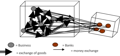
The free market economic system should be based on a dynamic agent-based growth. A dynamic agent-based growth is each individual’s capacity to produce real values. A macroscopic growth is the sum of individual dy-namic agent-based growth. A dydy-namic growth is based on eliminating surplus as a function of increasing market share and rise in unit prices, [23]. Dynamic growth is based on eliminating diminishing returns. All the above factors can be represented by the flow and the density of supply and demand. The flow and the density of de-mand represent endogenous adaptation of economic agents. The flow and the density of supply represent la-bor-technology interaction and the diminishing returns. 6) In a free market economy, economic activities1 should have a limited life span. Each economic activity should last as long as it produces real values. This is a response to flow and density of real demand that diminish in time. During the useful life of an economic activity, labor-machine productivity should stay positive but bounded. This implies that the flow and the density of supply are finite over time and should respond to real demand. The flow and the density of supply is a measure of labor-machine productivity. 7) A productive free market economy is an environment that allows for new ac-tivities that are created as a result of innovation from within the economic acac-tivities (innovation due to intelli-gent labor force) or from outside (individuals (consumer innovations)). 8) For the market to function efficiently it is necessary to separate small scale economy and large scale economy. Small scale economy refers to a system of small manufacturing and business. Large scale economy refers to a system of monopolies and oligopolies. It is assumed that oligopolies have large market shares that get larger in time. Whereas, small scale economies have fix market shares over time. 9) Each scale of economic activity makes up the two major layers, each major layer has many sub-layers, the function of which is to support and help more efficient functioning of each major layer. The support sub-layers are mainly banks. A system of small size banks sees to the investment needs of small scale economic activities. A system of large size banks sees to the investment needs of large scale eco-nomic activities. The two banking systems function in parallel. Figure 1, demonstrates the relationship between small scale economic activities and their corresponding banking system. As is shown by arrows, small scale businesses interact with each other through a supply chain, and capital lending, while they interact with banks through a system of lending/borrowing activities, where small businesses borrow limited capital with interest rates functions of the risk levels, and the amount of capital borrowed, [24].
[image:4.595.205.397.561.690.2]Figure 2demonstrates the relationship between oligopolies and large banks. As is shown by arrows, oligopo-lies do not interact with each other through a supply chain, and capital lending, but they interact with banks through a system of lending/borrowing activities, where they borrow unlimited capital with low interest rates.
Figure 1. Small scale activities economy.
Figure 2. Monopolistic and oligopolistic economy.
= Business = Banks
= exchange of goods = money exchange
34
An empirical data from the bank of England shows that the three-month annualized rate of growth of lending to large businesses picked up in the three months to May in 2014. The annual rate of growth of lending to both small and medium-sized enterprises (SMEs) remained negative, as is demonstrated in Figure 3 [24]. This could be explained by the lack of separation by size of the banking system.
3. Fundamental Theorems and Proofs
Three fundamental elements are identified from the literature in the theory of capitalism. These elements are: 1) demand (D) is not static but is rather a function of time (t),
(
D=Dt)
. 2) Supply (S) is also time dependent, andthus is referred to as real demand semi-responsive supply or (rdsrs),
(
S=St)
. 3) Labor is dynamic (timede-pendent), and evolves with time,
(
Γ = Γt)
. This section will start with the definition of several variables. Thefirst of these variables is real demand,
( )
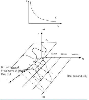
Dt . Real demand is a consequence of economic agent’s real needs andindividual innovating approach to solve problems in time (t). Individual innovation is defined as solutions found by economic agents to their problems as stochastic elements that lead to demand for new products or services. Induced demand is in contrast to real demand. Induced demand can be defined as a desire to consume not be- cause of a genuine need for a product but as a result of media and industry manipulations. Conventional demand is shown in Figure 4(a). In Figure 4(a), (D), is the demand curve, (Q) is the quantity demanded, and (P) is price. Conventional demand is static and does not vary with time (t). The real demand is time dependent
(
D=Dt)
,and does not have a regular pattern, and its shape reflects the attitude of economic agents. Real demand peaks up for a certain period of time as more and more people believe that the solution to their problem is the product in the market. At this point, it is monotonically increasing with positive slope.
( )
Dt peaks to its maximum afterwhich it goes down for a certain period of time towards zero demand, as the result of changes in the individuals’ tastes, choices, and preferences that change in time (t). The downward segment of the
( )
Dt is monotonicallydecreasing with negative slope. Zero real demand may last for a certain time, but this may not be a permanent condition. In time the same product may be the solution for another common problem; which would propel the real demand curve upwards, and the whole demand cycle starts all over again. Due to time dependent influences, real demand,
( )
Dt keeps the same pattern irrespective of price changes. This is shown in (3) dimensions (Q, P, [image:5.595.147.448.429.623.2]t), where (t) stands for time in Figure 4(b).
Figure 3. Lending to UK businesses, by business size. (a) Rate of grow in the stock of lending. Lending by UK MFIs, unless otherwise stated. Data cover lending in both sterling and foreign currency, expressed in sterling. Non seasonally adjusted. Further details are provided in the spreadsheet, available at:
(a)
[image:6.595.126.476.85.477.2](b)
Figure 4. (a)Conventional demand; (b) Real demand (Dt).
Figure 4(b)demonstrates the evolution of real demand
( )
Dt , with respect to price (P), and time (t). As isshown in Figure 4(b), real demand
( )
Dt peaks at a fixed price( )
P0 at time( )
t0 , where(
Dt0 =Q1max)
, and(
Q1max)
is the maximum quantity demanded at time( )
t0 .( )
Dt then fluctuates until it reaches zero,(
0)
1 =
t
D , at time
( )
t1 .( )
Dt peaks again(
Dt2 =Q2max)
, where(
Q2max)
is the maximum quantity demand-ed at time
( )
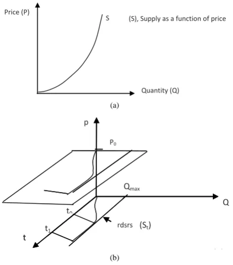
t2 . This process can go on for any finite time interval. Modeling of demand as a time dependent (stochastic) element seems to agree with consumer behavior in a laboratory environment, where fluctuations in demand for a given set of food products are concluded to be the result of time spent in doing the experimental tasks of product evaluation [25]. Conventional supply is shown in Figure 5(a).The real demand semi-responsive supply or (rdsrs) denoted by
( )
St imitates real demand approximately. Asreal demand
( )
Dt increases (rdsrs)( )
St increases; during the slowdown of real demand, (rdsrs) increases ata very slow rate, while real demand goes to zero, (rdsrs) stabilizes and stays constant. At zero real demand, (rdsrs) stops definitely. (rdsrs) has one significant feature, surplus or (excess supply) is finite. (rdsrs) satisfies a fixed percentage of the market demand. If real demand increases beyond maximum production plus surplus, then supplier will not raise production, rather he will continue at maximum production level for a period of time till real demand for the product diminishes irreversibly. At this point the real value of the product has reached zero, and it is time to stop production definitively.Figure 5(b), shows the (rdsrs) pattern.
D P
Q
Q
t
p
P0
Dt
Q1max Q2max Q3max
Real demand = Dt No real demand,
irrespective of price level (P0)
36
(a)
[image:7.595.184.415.83.345.2](b)
Figure 5. (a) Conventional supply; (b) Supply as a function of real demand.
As is shown in Figure 5(b), during interval
[ ]
0,t0 , and at a fixed price( )
P0 , (rdsrs)( )
St increasesmono-tonically till time
( )
t0 ,( )
St is at its’ maximum supply level(
Qmax)
which corresponds to the maximum level of real demand( )
Dt . During the fluctuations in( )
Dt ,( )
St remains fixed at(
Qmax)
. At time( )
t1 ,( )
St drops to zero, when real demand( )
Dt is at (0). This cycle repeats itself, if real demand goes through anew cycle. Empirical studies seem to confirm the behavior of (rdsrs)
( )
St . In Figure 6, the supply ofphysi-cians per 100,000 population stayed fixed for a certain period irrespective of fluctuations in demand [26]. Finally, labor is redefined as intelligent labor,
( )
Γι . Intelligent labor is synonym for dynamic technology.Dynamic technology refers to the level of intellectual prowess, strategic maneuvering, movement and mental and physical agility of an economic agent. High tech machinery, tools and instruments are referred to as physical technology. Physical technology can be considered as static technology. Physical technology relies on human innovation, thus is static at any interval of time. In contrast, dynamic technology is considered to be able to self- improve continually in time and thus dynamic. The three variables, real demand,
( )
Dt , real demand semi-res-ponsive supply,
( )
St , and intelligent labor,( )
Γt , are used in the proofs of the theorems below. It should benoted that in the proof of Theorem 1. Some notions from the traffic flow theory are borrowed. Real demand
( )
Dt is taken to be analogous traffic on a road, [27]. This analogy is appropriate since the behavior of driverswhen choosing a road is analogous to consumer preference as it is complete, reflexive and transitive. The road itself is analogous to the real demand semi-responsive supply,
( )
St . This is an appropriate analogy since a roadis a service supplier, and allows for a range of demand fluctuations, but has a fixed maximum supply capacity.
Theorem 1: Given that real demand
( )
Dt exists and it is periodic; then real demand semi-responsive supply(rdsrs)
( )
St should be bounded.Proof: Real demand
( )
Dt can be expressed in terms of flow and density. The flow of demand2
is the quanti-ty demanded of any product per unit of time. The flow of demand is denoted by qd
( )
i t, , (i) indicates product (i), where(
i=1,,n)
, and (t) stands for time. The flow of demand is given by:( )
, i 1, ,d
Q
q i t i n
t
= ∀ = (1)
Quantity (Q) Price (P)
S (S), Supply as a function of price
p
Q
t
P0
rdsrs
Qmax
(b)
Q
t
P0
rdsrs
Qmax
(b)
t0
t1 (St)
Figure 6. Empirical evidence of time dependent supply.
( )
Qi is the quantity demanded of good (i) per unit of time (t). The density of demand is the quantity ofprod-uct (i) demanded per square kilometers. The density of demand is denoted by ρd
( )
i L, 2 , is demand per square kilometers( )
L2d . The density of demand is given by:( )
2 2, i 1, ,
d
d
Q
i L i n
L
ρ = ∀ = (2) The speed
( )
νd with which demand( )
Dt propagates is formulated as the propagation of demand bykilo-meter
( )
Ld per unit time (t):d d
L v
t
= (3) The relationship between the flow and the density of demand is given by:
( )
( )
2, ,
d d d
q i t =ρ i L ×v (4) The flow of demand qd
( )
i t, has (7) phases over time. These phases represent the attitude and strategic ap-proach of economic agents towards demand. the attitude and strategic apap-proach of economic agents is the sto-chastic (time dependent) elements involved in having demand such as taste, choice, preferences as they are acyclic, transitive, have a semi order property, and are complete. A phase is defined as the level of demand at time (t). The occurrence of a demand phase in time should have continuity, convexity, homogeneity, and trans-lation-invariance properties. Given the prerequisites, phase (1) represents a situation where the number of goods demanded increases rapidly in time. During phases (2) & (3), the number of goods demanded increases mod-erately. In phase (4), the number of goods demanded decreases modmod-erately. At this stage two possibilities arise; either demand increases or decreases. Phase (5) represents the possibility that demand increases. This phase is unstable and can only occur during a short period. Phase (6) represents the other possibility that the number of goods demanded drops to zero. Phase (7) represents a period when the number of goods demanded stays at zero. If the consumption of a product becomes the solution of certain economic problems for a number of agents, it is then possible to have a repetition of phases (1), (2), (3), (4), (6), and (7) over time. The probability of occurrence of phase (5) is considered small and thus is excluded from cyclical considerations. The many phases of the flow of demand are demonstrated in Figure 7.The relationship between the flow and the density of demand is demonstrated in Figure 8. In phase (1) of
38
[image:9.595.182.424.240.412.2]Figure 7. Different phases of the flow of real demand.
Figure 8. Flow vs. density of demand.
mand increases moderately, while the density decreases. This is an indicator of a general slowdown in demand. In phase (6), both the flow and the density of demand decrease rapidly. This implies that the slowdown in de-mand intensifies. In phase (7), both the flow and the density of dede-mand are null. Dede-mand ceases to exist. This relationship between the flow and the density of demand is adopted from the traffic flow theory. Why would demand for a product behave in the same way as the flow of traffic on a road segment? Consider the road seg-ment as a product that is consumed by users (drivers). It is shown through various studies and data collected from various sites at different times of day, that traffic behaves in phases. This can be translated as the change in demand for a product that is a road segment. The assumption is that demand behaves in the same manner as traf-fic demand for the use of a road segment.
The same phase patterns can be observed if the density of demand ρd
( )
i L, 2 is traced out in time. This is shown in Figure 9.Real demand semi-responsive supply (rdsrs)
( )
St can be defined in the same quantitative manner as demand.The flow of (rdsrs), q i j ts
(
, ,)
is defined as the quantity of good (i) exchanged for good (j),( )
Qij , per unittime (t). This is expressed as follows:
(
, ,)
ij 1, , ; 1, , ;s
Q
q i j t i n j m i j
t
= ∀ = = ≠ (5)
The density of (rdsrs), ρs
(
i j L, , 2)
is defined as the quantity of good (i) exchanged for good (j) per square kilometer,( )
L2s . The density of (rdrs) is an indicator of the preference for good (i) over good (j).(
2)
2
, , ij 1, , ; 1, , ;
s
s
Q
i j L i n j m i j
L
ρ = ∀ = = ≠ (6)
In the same manner the speed of (rdrs),
( )
νs is given by:( )it qd ,
(t) Phase 1
Phase 2 & 3
Phase 4 Phase 5,6
Phase 7
Phases repeat over time
( )
i,L2d
ρ
( )
it qd ,Phase 1
Phase 2
Phase 3
Phase 4 Phase 5
Figure 9. Density of demand vs. time.
s s
L v
t
= (7)
( )
vs is the speed with which good (i) is exchanged with good (j) per unit of time (t).( )
Ls is the radius inkilometer from the point of production or distribution. The speed of (rdsrs),
( )
vs is a measure of how fast good(i) is exchanged with good (j). The relationship between the flow, q i j ts
(
, ,)
and the density of (rdrs),(
2)
, ,
s i j L
ρ is expressed as:
(
)
(
2)
, , , ,
s s s
q i j t =ρ i j L ×v (8) Following the analogy with the traffic flow theory, the flow of (rdsrs), q i j ts
(
, ,)
demonstrates several phas-es in time (t). The (3) phases of q i j ts(
, ,)
are shown in Figure 10. Phase (1) is exactly similar to phase (1) of the flow of demand, qd( )
i t, . In phase (1), q i j ts(
, ,)
follows the behavior of qd( )
i t, . Phase (2) correspondsto phases (2), (3), & (4) of the flow of demand, qd
( )
i t, . During phase (1), surplus is accumulated. The surplus plus a moderate supply level will see to the needs of phases (2), (3), and (4) of qd( )
i t, . Phase (3) of q i j ts(
, ,)
corresponds to phases (6) & (7) of the flow of demand, qd
( )
i t, .The speed-flow and speed-density relationship is demonstrated in Figure 11. The speed of (rdsrs) is at maxi-mum when the density of (rdsrs), ρs
(
i j L, , 2)
is zero. As the density,(
)
2 , ,
s i j L
ρ increases the speed
( )
vsgoes down until at maximum density, it reaches zero. This means that supply of good (j) has gone up. The speed
( )
vs goes down as the flow of supply, q i j ts(
, ,)
goes up. Once maximum flow is reached, the processre-verses itself and
( )
vs goes down until it reaches zero.Figure 12 shows how the flow of demand, qd
( )
i t, , and the flow of (rdsrs), q i j ts(
, ,)
are related to eachother.
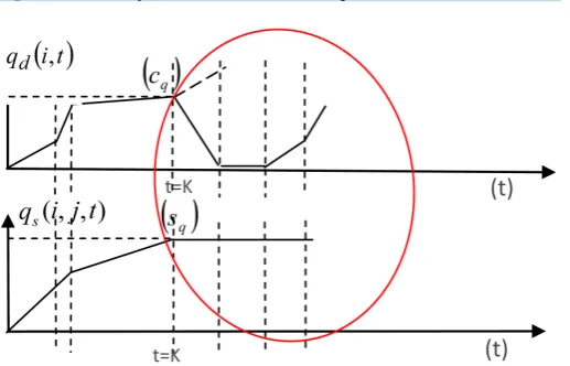
From Figure 12, it is shown that the flow of demand, qd
( )
i t, reaches its maximum at time (t = K). This is mathematically expressed as:( )
, limt K qd i t cqt
→ ∂
=
∂
(9) Given Equations [9], and [4], the density of demand, ρd
( )
i L, 2′
at point
( )
cq can be calculated. Given thatthe flow of demand is at its maximum point
( )
cq , then the density of demand( )
2 ,
d i L
ρ ′ is minimum at point
( )
cq , given a fixed speed,( )
vd .( )
( )
( )
( )
( )
2
2
2 2
,
,
, , ,
q d d
q d
d
q
d d d
i L v
c
c i L
v
i L i L q i t c
ρ
ρ
ρ ρ
′
= ×
′ =
′ ≤ ∀ <
(10
( )
2 ,L id
ρ
(t)
Phase 1 Phases 2 & 3
Phase 4
Phase 5
40
[image:11.595.172.431.382.548.2]Figure 10. Flow of (rdsrs) vs. time.
Figure 11. Density and flow of (rdsrs) vs. speed.
Figure 12. Relationship between the flow of demand and the flow of (rdsrs).
From Figure 12, the flow of (rdrs), q i j ts
(
, ,)
reaches its maximum( )
sq , at time (t = K). This ismathe-matically expressed as:
(
, ,)
limt K q i j ts sq
t
→ ∂
=
∂
(11) Surplus is denoted by
( )
Ψ . Surplus is defined as the difference between supply and demand,(
)
(
Ψ = ∆ D St, t)
. The maximum flow of demand( )
cq is equal to the maximum flow of supply( )
sq ,(
cq =sq)
, when surplus(
Ψ =0)
. If this was not true, two cases could occur: 1) The maximum flow of realdemand is greater than
( )
cq ,(
)
h q qc <c . 2) It is less than
( )
cq ,(
)
h q qc >c .
( )
chq is the maximum flow of(t)
) , , (i jt qs
Phase 1
Phase 2 Phase 3
) , , (i j t qs )
, , (i j L2
s
ρ
demand other than
( )
cq . In case (1), the maximum flow of (rdrs),( )
sq is less than( )
h qc ,
(
sq <cqh)
, if(
h)
q q
c <c , and surplus
( )
Ψ is less than zero(
(
h)
0)
q q
s c
Ψ = ∆ − < . In case (2), the maximum flow of (rdrs),
( )
sq is greater than( )
h qc ,
(
sq >cqh)
, if(
)
h q qc >c , and surplus
( )
Ψ is positive(
Ψ = ∆(
sq−cqh)
>0)
. In case (1), since(
Ψ = ∆(
sq−cqh)
<0)
implies that(
sq=0)
, it is in contradiction with the assumption that( )
sq is maximum. In case (2), since(
(
)
0)
h q qs c
Ψ = ∆ − > , implies that
(
sq>cq)
, which is in contradictionwith the assumption that
(
cq=sq)
at maximum. Therefore,( )
sq is bounded at(
cq =sq)
.□Theorem 2: Given that
( )
Dt exists and has multiple phases, and( )
St is semi-responsive and bounded,(
St∈ 0,cq)
, then( )
St is finite in time,(
limt→T( )
St ≤cq)
.Proof: Let (T) be a time horizon, and let (T) be divided into (N) equal intervals of length
(
∆ ≥t 0)
,(
)
(
T= ∆ ∆t1, t2,,∆tN)
. Let(
qd(
i,∆tτ)
≥0)
during each(
∆tτ;τ=1, 2,,N)
. Let(
qd(
i,∆tτ)
≥0)
be a stepfunction defined by Equation [12]:
(
)
( )
(
) ( )
( )
1 1 1 , sup 1 0 i i n Nd q q
T i
q i t c t c t t
t T
t
t T
τ τ τ τ
τ τ τ τ τ χ χ − ∈ = = ∆ = ∆ − ∆ ⋅ ∆ ∆ ∈ ∆ = ∆ ∉
∑∑
(12)The step function
(
qd(
i,∆tτ)
)
is shown in Figure 13. During each interval two possibilities can occur:1) cqi
( )
∆tτ −cqi(
∆tτ−1)
≤ε; ∀∆ ∈tτ T,∀ ∈i(
1,,n)
for any(
ε >0)
,2) cqi
( )
∆tτ −cqi(
∆tτ−1)
≥ε; ∀∆ ∈ ∀ ∈tτ T, i(
1,,n)
.If (1) occurs, then
( )
(
1) ( )
1 1 sup i i n N q q T i
c tτ c tτ tτ
τ τ
χ − ∈ = =
∆ − ∆ ⋅ ∆ < ∞
∑∑
is bounded, and qd(
i,∆tτ)
has a unique maximum equal to( )
cq . By Theorem 1, the maximum flow of supply( )
sq is bounded and equal to( )
cq ,(
sq=cq)
, and since( )
cq is the maximum for the time horizon (T), then( )
sq is bounded and thus finite intime. If (2) occurs, then
( )
(
1) ( )
1 1 sup i i n N q q T i
c tτ c tτ tτ
τ τ
χ − ∈ = =
∆ − ∆ ⋅ ∆ > ∞
[image:12.595.86.535.332.722.2]∑∑
is not bounded, and thus qd(
i,∆tτ)
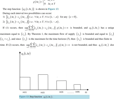
doesFigure 13. Step function qd
(
i,∆tτ)
. ...∆t(1) ∆t(2) ∆t(3) ∆t(N) (t)
( )
i t42
not have a unique maximum, which implies that
( )
sq is not bounded. This is in contradiction with the resultsof Theorem 1. Thus (2) cannot occur. (1) is the only possible case, and thus
( )
sq is bounded and finite in time,( )
(
limt→T St ≤cq)
. □Theorem 3: Given that supply of any given product is semi-responsive, and bounded, and if the supply of the
next product demonstrates the same attributes, and that there is always another product with the same supply characteristics and this process is repetitive, then growth occurs and is positive and monotonically increasing.
Proof: Let
(
g g1, 2,,gM)
be (M) goods existing in a market during time (T). Let the flow and density ofdemand and supply for each one good be positive during each interval
(
∆ =tτ[
tτ−1,tτ]
∈T;τ =1, 2,,M)
,(
)
(
)
(
qd gi,∆tτ >0 ;∀ =i τ)
,(
(
)
)
2
, 0;
d g Li t i
τ
ρ τ
∆ > ∀ = , and
(
qs(
g gi, j,∆tτ)
> ∀ ≠0; i j,∀ =i τ)
,(
)
(
qs gj,gi,∆tτ >0;∀ ≠ ∀ =j i, j τ)
,(
(
)
)
2
, , 0; ,
s g g Li j t i j i
τ
ρ τ
∆ > ∀ ≠ = ,
(
(
)
)
2
, , 0; ,
s g g Lj i t j i j
τ
ρ τ
∆ > ∀ ≠ = . If limt tτ
(
d(
g Li, 2)
t)
0; iτ
ρ τ
→ ∆
= ∀ =
, and
(
(
)
)
2
, 0;
d j
t
g L j
τ
ρ τ
∆ > ∀ = , then
(
)
(
lim ( , , ) j; ,)
t→tτ q gs j gi ∆tτ =sq ∀ ≠ ∀ =j i j τ , and
(
(
)
(
)
)
2 2
, , , , ; ,
s g g Lj i t s g g Li j t j i j
τ τ
ρ ρ τ
∆ > ∆ ∀ ≠ = . If
(
)
(
2)
limt→tτ ρd g Li, ∆tτ 0; i τ
= ∀ =
, then the marginal flow and density of good
( )
gi ,(
, ,)
limt t s i j 0; ,
q g g t
i j i
t τ τ τ → ∂ ∆ = ∀ ≠ ∀ = ∂
, and
(
)
2
2 , ,
lim 0; ,
s i j t
t t
g g L
i j i L τ τ ρ τ ∆ → ∂ = ∀ ≠ = ∂
, are zero,
otherwise qs
(
g gi, j, t)
0; i j, i tτ
τ
∂ ∆
> ∀ ≠ ∀ =
∂ ,
(
)
2 2 , , 0; ,s g g Li j t
i j i L τ ρ τ ∆ ∂
> ∀ ≠ =
∂
, the marginal flow and
density of good
( )
gi are positive. If(
, ,)
0; ,
s i j
q g g t
i j i
t
τ
τ
∂ ∆
> ∀ ≠ ∀ =
∂
, is true, growth per interval is
de-fined as
(
)
1
, , d
t
s i j q
t
q g g t
s t t τ τ τ − ∂ ∆ = ∂
∫
. Since
(
sq>0)
, then growth is positive. Growth for the entire period(T) is the sum of growth per interval, and is thus positive and monotonically increasing,
1 , 0 M i i q q i
G s s
=
= ∀ >
∑
. □Theorem 4: Given that real demand exists, and supply is semi-responsive, bounded, and finite in time, then
bank liquidity should be bounded.
Proof: Let time (T) be divided into (N) equal time intervals
(
tτ =(
t t1, ,2,tN)
)
. Let the total number of labor( )
Γι be equal to( )
Mι ,(
Γ Γ =ι; ι 1, 2,,Mι)
. Bank liquidity is the sum of savings. Savings (S) is formulatedas
(
S=(
[
I−C]
+ Π)
)
. Income (I) per interval is equal to1 m I I ι ι ι Γ Γ = =
∑
, where( )
IΓι is the income of each labor, and( )
mι is the total fixed number of labor per square kilometer. Let the density of labor3 be formulatedas
(
2)
12 , m L L ι ι ι ι ι
ρ Γ =
Γ
Γ
Γ =
∑
, be the number of labor per square kilometers at any interval( )
tτ .( )
IΓι per labor isthen equal to
(
(
2)
)
,
IΓι =ρΓι Γι L ×Pι , where price per unit of labor
( )
Pι is set fixed. Consumption (C) is equalto the density of demand,
(
( )
2)
, ; 1, 2, ,
d i L i n
ρ = , times the price of good (i),
( )
pi ,( )
2 1 , n d i i
C ρ i L p
=
= ×
∑
.Profit
( )
Π is formulated as the density of supply ρs(
i j L, , 2)
multiplied by the price of good (i),( )
Pi ,(
)
(
2)
1
, , i
s
n
i
P i j L
ρ
=
×
∑
, where( )
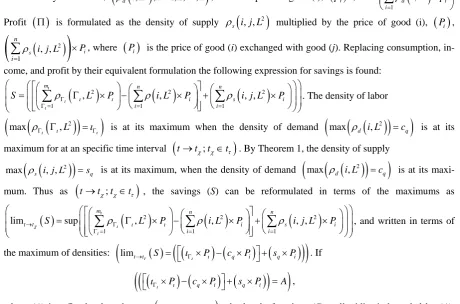
Pi is the price of good (i) exchanged with good (j). Replacing consumption, in-come, and profit by their equivalent formulation the following expression for savings is found:
(
2)
( )
2(
2)
1 1 1
, , , ,
m n n
i s i
i i
S L P i L P i j L P
ι ι ι
ι ι
ρΓ ρ ρ
Γ = = =
= Γ × − × + ×
∑
∑
∑
. The density of labor
(
)
(
)
(
2)
max ρΓι Γι,L =ιΓι is at its maximum when the density of demand
(
max(
ρd( )
i L, 2)
=cq)
is at itsmaximum for at an specific time interval
(
t→tχ;tχ∈tτ)
. By Theorem 1, the density of supply(
)
(
2)
max ρs i j L, , =sq is at its maximum, when the density of demand
(
max(
ρd( )
i L, 2)
=cq)
is at itsmaxi-mum. Thus as
(
t→tχ;tχ∈tτ)
, the savings (S) can be reformulated in terms of the maximums as( )
(
2)
( )
2(
2)
1 1 1
lim sup , , , ,
m n n
t t i s i
i i
S L P i L P i j L P
ι
χ ι
ι
ι ι
ρ ρ ρ
→ Γ
Γ = = =
= Γ × − × + ×
∑
∑
∑
, and written in terms of
the maximum of densities:
(
limt t( )
S(
(
P)
(
cq Pi) (
sq Pi)
)
)
τ ιι ι
→ = Γ × − × + × . If
(
)
(
) (
)
(
)
(
ιΓι×Pι − cq×Pi + sq×Pi =A)
,where (A) is a fixed value, then as
(
t→tχ;tχ∈tτ)
, the level of savings (S) or liquidity is bounded by (A),( )
(
limt→tχ S =A)
. This means that during any time interval other than( )
tτ ,(
( )
St <A)
. □Theorem 5: Monopolistic and oligopolistic based economic activities are in conflict with small
manufactur-ing and service activities.
Proof: The theorem is proved by showing that there are fundamental differences between demand and supply of oligopolies and small business activities. It is these differences that create incompatibility between the two types of systems. On the demand side, let’s start the comparison by defining the flow of demand
( )
,O
O i
d
Q
q i t
t
=
as
the demand for good (i) produced by oligopolies per unit of time, and the density of demand
( )
2 2 , O O i d Q i L L ρ = as the demand for good (i) produced by oligopolies per square kilometer. By definition oligopolies take a large share of the market. This is due to targeting high density population areas, controlling prices, and replacing labor with static technology. Therefore, the flow and density of demand of oligopolies are greater than that of small producers,
(
qdO( )
i t, >qd( )
i t,)
, and(
( )
( )
)
2 2
, ,
O
d i L d i L
[image:14.595.83.544.103.407.2]ρ >ρ . This inequality is graphically demonstrated in
Figure 14.
In Figure 14,
( )
qOd is the flow of good (i) produced by oligopolies,( )
qd is the flow of good (i) producedby small producers. The oligopoly marginal flow of demand is positive and increases in time
( )
,lim
O d
t T q
q i t
t → ∂ = Λ ∂
where
(
O( )
,( )
, 0)
q qd i T qd i T
44
Figure 14. Oligopoly flow of demand vs. small producers.
( )
,limt T d 0
q i t t → ∂ = ∂
. Substituting for the marginal flow of demand of small businesses,
(
( )
, 0)
O
q qd i T
Λ = ≥ .
Comparison between the oligopolys’ and the small producers’ density of demand is shown in Figure 15. The density of demand of oligopoly is linearly increasing while the density of demand of small producer reaches a maximum and then reverses direction and goes to zero.
In Figure 15,
( )
ρOd is the density of good (i) produced by oligopolies,( )
ρd is the density of good (i)produced by small producers. Since the oligopoly marginal flow of demand is monotonically increasing in time, the oligopoly marginal density of demand must be monotonically increasing in time,
( )
2 2 , lim O d t T i L L ρ ρ → ∂
= Λ
∂
,
with
(
Λ =ρ ρdO( )
i L, 2 −ρd( )
i L, 2 ≥0)
. Given that( )
,limt T d 0
q i t t → ∂ = ∂
, then
( )
2 2 ,limt T d 0
i L L ρ → ∂ = ∂ ,
and
(
O( )
, 0)
d i T
ρ ρ
Λ = ≥ .
On the supply side, the flow
(
, ,)
O ij O
s
Q q i j t
t
=
, and the density of supply
(
)
22
, , ij
O s
Q i j L
L
ρ
=
of
oligopo-lies and small producers behave in very distinct ways from each other. As is shown in Figure 16, the flow
(
)
(
qsO i j t, ,)
and the density(
(
)
)
2
, ,
O
s i j L
ρ of supply of oligopoly increase linearly, while those of small pro- ducers increase and then stay fixed at maximum, since supply is bounded and finite in time. This can also be seen from the comparison of marginal costs of oligopoly and small producer. In Figure 17, small producers have a higher marginal cost (Cm2) at the beginning of their operation, when the density of supply
(
(
2)
)
, ,
s i j L
ρ
is low. (Cm2) goes down as the density of supply
(
(
, , 2)
)
s i j L
ρ goes up, and eventually goes up again reacting to fluctuations in density of supply. The marginal cost (Cm1) of oligopolies, is higher than small businesses, but due to the economies of scale, the marginal cost (Cm1), goes down and stays down as the density of supply
(
)
(
O , , 2)
s i j L
ρ of oligopolies goes up. The same applies to labor and investment costs. InFigure 18, the differ-ences in labor costs are demonstrated. For the oligopolies, the cost of labor goes down as more labor is replaced by static technology, while small businesses maintain a level of labor. In Figure 19, the differences in invest-ment levels of oligopolies and small businesses are shown. In both Figure 18 and Figure 19, (1) Stands for small businesses, and (2) stands for oligopolies. Oligopolies have higher initial marginal costs (Cm1) which get smaller as time goes on. The oligopoly marginal flow of supply is positive and increases in time
(
, ,)
lim
O s
t T q
q i j t
t δ → ∂ = ∂ (t) i Q
( )
qd( )
O dq
Figure 15. Oligopoly density of demand vs. density of demand of small producer.
Figure 16.Oligopoly flow and density of supply vs. small producer
flow and density of supply with respect to time (t) and space
( )
L2 .qs ij
Q
(t)
ρs
ij
Q
(L2)
qO
s
[image:16.595.172.426.381.685.2]46
[image:17.595.193.406.238.445.2]Figure 17. oligopoly marginal cost of production of vs. small producers’ marginal cost of production with respect to the density of supply of small businesses, and oligopolies.
Figure 18. Differences in labor pattern of small business-es and oligopolibusiness-es.
Figure 19. Differences in investment between small busi-nesses and oligopolies.
(
)
(
2)
, ,jL i
s ρ
Cost
Cm1
Cm2
(
)
(
2)
, ,jL i
O s ρ
1
2
labor
Cost
Dynamic technology
1 2
[image:17.595.193.402.481.697.2]where
(
δq = qsO(
i j T, ,)
−qs(
i j T, ,)
≥0)
. This is due to improvements in the production of good (i), using static technology. The small producers’ marginal flow of supply is zero in time, limt T s(
, ,)
0q i j t t → ∂ = ∂ .
Marginal flow of supply follows the same trend as the Marginal flow of demand. Substituting for the marginal flow of supply of small businesses,
(
Λ =s qOs(
i j T, ,)
≥0)
.Since the oligopoly marginal flow of supply is monotonically increasing in time, the oligopoly marginal den-sity of supply must be monotonically increasing in time,
(
)
2 2 , , lim O s t T
i j L
L ρ ρ δ → ∂ = ∂ , with
(
) (
)
(
2 2)
, , , , 0
O
s i j L s i j L
ρ
δ = ρ −ρ ≥ . Given that limt T s
(
, ,)
0q i j t t → ∂ = ∂
, then
(
2)
2 , ,
limt T s 0
i j L
L ρ → ∂ = ∂ ,
and
(
(
2)
)
, , 0
O s i j L
ρ
δ = ρ ≥ . In time given, the expansion of flow and density of demand and supply of oligo-polies, it becomes difficult for small businesses to reenter the market, or for new businesses to enter. □
Theorem 6: Given the assumed patterns of the flow and the density of demand and supply of small and large
economic operations, the two systems should function separately, but in parallel.
Proof: Let good (i) be produced by small businesses, and good (i') be produced by oligopolies. Let total mar- ket demand be equal to (M). Let the quantity of good (i) produced by small businesses be
( )
Qi , and the quantityof good (i') produced by oligopolies be
( )
Qi′ , then(
M =(
Qi′+Qi)
)
. If(
i=i′)
, then(
Qi′=(
M −Qi)
)
,and as the flow and density of demand and supply of oligopolies increases, the flow and density of demand and supply of small businesses diminishes, until at time (T), where (T) is equal to one demand cycle, the quantity of good (i') be produced by oligopolies becomes equal to the total market demand (M),
(
M =Qi′)
. This isdemon-strated in Theorem 5. If
(
i≠i′)
, then there exists a total market demand for (i),( )
M , and a total market de-mand for good (i'),( )
M′ , such that(
(
MM′ =)
0)
, and(
(
MM′)
=M +M′)
. The evolution of the flow and the density of demand and supply of either oligopoly, or small business have no impact on each other. Pa-rallel operation of the two systems of small businesses and oligopolies, creates higher growth. From Theorem 3, growth due to the operation of small businesses is a function of the flow of supply, when it is at maximum. Therefore, it is positive. Growth due to the operation of oligopolies is positive, since the marginal flow of supply is positive and increasing, as is shown in Theorem 3. Let growth due to small businesses be denoted by(
Gs >0)
, and let growth due to oligopolies be denoted by(
GsO>0)
. Total growth( )
G is then equal to(
)
O s s
G=G +G , if both small businesses and oligopolies function in parallel. If only one of the two systems functions, the growth is always less than the growth reached by the parallel operation of the two systems together,
(
G>Gs)
, and(
O)
s
G>G , both growths being equal, the sum of the two growths is always greater, than its’ individual ele-ments. □
4. Parallel-Multi-Layer Capitalism (Pmlc) as a Natural Outcome of the
Theorems Introduced
48
supply in the form of asset prices and other financial instruments. 3) This system is dependent on an unbounded demand and supply in an asymmetric market. Prominent characteristics of the German export model are: 1) This system is based on asymmetric market mechanisms. 2) Demand is an increasing function of asymmetric infor-mation. 3) A large banking system based on stock market activities. 4) oligopolies with peripheral subsidiaries. 5) This system is dependent on an unbounded and monotonically increasing demand and supply in an asymmetric market. The reliance of all (3) economic systems on asymmetric markets, asymmetric information, and financial mechanisms render these systems vulnerable to economic crisis, [28]-[30]. Asymmetric markets, and asymme-tric information introduces random effects in demand and supply. They can cause unanticipated inflationary, or deflationary prices that cause contractions in the pattern of demand and supply. Asymmetric information can cause adverse selection problems that weakens the financial market mechanisms and creates instability in terms of liquidity crisis.
The PMLC model is sustainable because it is based on bounded market share or bounded demand, bounded and stochastically constrained supply, and separation of small and large scale systems. Bounded demand and supply mean free entry of small businesses into the market. This system reduces the risks outlined above for the (3) existing economic systems. These risks are functions of the dependency of the economy on large market shares or demand. The Parallel Multi Layer system guarantees continuous employment and thus long term de-mand and supply of goods. The real value of any good has a finite duration; although dede-mand is sustainable, demand for any single good is finite and disappears in time. Demand and supply are introduced as space-time dependent variables. Three main notions are introduced to give more depth to these variables. These notions are the flow, the density, and the speed of demand and supply. The flow of demand and supply is a measurable quantity given observational data. It concretizes the time dependency of demand and supply. The density is a measurable quantity given observational data and concretizes the space dependency of the two variables. The speed of propagation is a concrete way of showing space-time correlation of demand and supply. The three no-tions of the flow, density, and speed capture the non-linearity of demand and supply and their bounded nature in time. Since demand and supply are bounded, asymmetric markets, and asymmetric information cannot create discontinuities.
Demand exists and is nonlinear with multiple phases, that constitute a cycle. Supply is semi-responsive and bounded and finite in time. Bounded and finite in time supply reduces production costs by reducing excess supply. It encourages free entry of economic activities that create real values for which real demand exists. Each economic activity plans for an optimal operation period that corresponds to the real demand cycle. Each eco-nomic activity encourages and promotes the next generation of ecoeco-nomic activities through maintaining a bounded and finite supply level. Since growth is the function of the flow of supply, then given that supply of any given product is semi-responsive, and bounded, and finite in time, and the supply of the next product has the same attributes, and there is always another product with the same supply characteristics and this process is cyc-lic, then growth is positive and monotonically increasing. Bounded and time finite supply, assure positive and monotonically increasing growth which in turn assures a dynamic technology base or labor. Dynamic technolo-gy base or labor is a conduit for smart, spontaneous, and productive innovations that assure entry of new prod-ucts into the market.
A fundamental layer in the PMLC system is the banking system. Within the PMLC, small and large banks work in complete separation. The liquidity base of small banks is assured by the revenue produced by small and large scale economic activities respectively. Small scale banks set their own interest rates which are based on the risks involved. Bounded and finite supply, lower excess supply, and limited investment requirements, result in bounded profit levels. As a result small bank liquidity is bounded. This lowers the lending risks and significantly eliminates the adverse selection problem due to asymmetric information and asymmetric market mechanism. Large scale banks work exclusively with large scale economic activities and their interest rates are determined by central banks. This assures the sustainability of the large banking system.
5. Conclusions
A new model is introduced. The aim is to provide a basis for an economic structure that can be sustained given the non-linear nature of demand and supply. Many definitions are given to prepare a proper setting for the theo-rems that are introduced later. These theotheo-rems are meant to provide a structural framework for an economic system. This economic system is called Parallel-Multi-Layer Capitalism, or (PMLC). This name is chosen due to the fact that the economic structure proposed is based on the separation of small and large economic activities. Each type of activity is considered to be an economic layer, and since all layers operate within the framework of free competition, in the case of small businesses, and regulated competition in the case of monopolies, and oli-gopolies, they are considered to operate in a capitalistic system. In (PMLC), the major driving force is demand. Demand is the result of the needs of an intelligent and rational consumer that seeks to find solutions to problems that relate to his/her living conditions. Therefore, these needs are time and space dependent and so are the solu-tions. Solutions translate into real demand which is time dependent. Real demand is nonlinear and cyclic. De-mand has a local maximum, and a local minimum during each cycle period.
The real value of a product is the degree of appropriateness, and usefulness of the product to the solution of consumer problems. A significant characteristic of small producers is their supply pattern. Supply of any product is bounded and finite in time. Each business activity keeps his share of the market fixed irrespective of fluctua-tions in demand. As demand increases supply increases, but it fixes itself at a local optimum of demand, thus eliminating the excess supply problem. This way whatever slack demand there is in the market is picked up by another small producer that will follow the same pattern of supply. It is a sure strategy for allowing the entries of new small producers in the market. Each business in the market decides on a fixed period of operational time. The advantage is that they can keep their costs manageable. The marginal, total, and average costs are reasona-bly incremented over time. The variable costs are stable during the life of the business. Productivity remains at its highest level during this period. Meanwhile, the next generation of goods mature to the point where they can enter the market. The PMLC system also allows for a parallel system of large scale operations. The condition imposed is that large economic activities should provide for services and create industries that differ from those of small businesses. Banks are also separated to serve small and large economic activities. The main difference is the liquidity base. For small banks the liquidity base is the savings of individuals and small producers’ profits. Their lending policy is based on interest rates as a function of risk. Limited profits and savings assure low level lending risks. Large banks have large liquidity base. They rely on large scale economic activities to secure their money supply. Their lending policy is based on interest rates set by central banks. Time will tell if PMLC model marks the maturation age of capitalism.
References
[1] The Economist. 21st-27th February 2009.
[2] Wallerstein, I. (1979) Aufstieg und zukünftiger Niedergang des kapitalistischen Weltsystems: Zur Grundlegung ver gleichender Analyse. In: Senghaas, D., Ed., Kapitalistische Weltökonomie: Kontroversen über ihren Ursprung und ihre Entwick lungsdynamik, Suhrkamp Verlag, Frankfurt am Main, 31-67.
[3] Althusser, L. (1978) Le capital. Maspero Publishing, Paris.
[4] Beckert, J. (2012) Capitalism as a System of Contingent Expectations: Toward a Sociological Micro Foundation of Po-litical Economy. Max-Planck-Institut für Gesellschaftsforschung, Köln.
[5] Walras, L. (1954) Elements of Pure Economics. Routledge Publishing, Cornwall.
[6] Eatwell, J., Milgate, M. and Newman, P. (1987) Walras’s Theory of Capital. The New Palgrave: A Dictionary of