Munich Personal RePEc Archive
Vulnerability to asset-poverty in
Sub-Saharan Africa
Echevin, Damien
Sherbrooke University, CRCELB, CIRPÉE
2011
Online at
https://mpra.ub.uni-muenchen.de/35660/
Vulnerability to Asset-Poverty in Sub-Saharan
Africa
Damien Echevin*
Abstract
This paper presents a methodology to measure vulnerability to asset-poverty. Using
repeated cross-section data, age-cohort decomposition techniques focusing on second-order
moments can be used to identify and estimate the variance of shocks on assets and,
therefore, the probability of being poor in the future. Estimates from the Ghana Living
Standard Surveys show that expected asset-poverty is a reliable proxy for expected
consumption-poverty. Applying the methodology to nine Demographic Health Surveys
countries, urban areas are found to unambiguously dominate rural areas over the
uni-dimensional distribution of expected future asset-wealth, as they also generally do over the
bi-dimensional distribution of present asset-wealth and expected future asset-wealth.
Keywords: vulnerability; poverty; wealth; pseudo panel; stochastic dominance; Africa.
JEL Numbers: D12; D31; I32; O12; O15.
1. INTRODUCTION
Over the past few years, the measurement of vulnerability has gained renewed
interest. Since at least the publication of the World Development Report 2001―and the
WDR 2010 more recently―development economists have been trying to figure out the
consequences and policy implications of measuring vulnerability to risks and shocks (be
they economic, climatic, etc.) in lieu of only considering more conventional poverty
indices.1 In particular, since both the poor and the non-poor can be vulnerable to shocks,
social security or safety nets should benefit a larger population than the one currently
targeted by poverty alleviation programs and assistance to the poor.
Various approaches to vulnerability measurement have been proposed in the
literature as different definitions have emerged.2 Vulnerability to poverty can first be
defined as a probabilistic concept: it is the risk of falling into poverty when one’s income or
consumption falls below a predefined poverty line. This calls for a quantitative approach to
vulnerability that implies estimating a probability as well as selecting a poverty line.3 In
order to estimate such a probability, Chaudhuri et al. (2002) proposed to estimate the
expected mean and variance in consumption using cross-sectional data or short panel data.
As in Pritchett et al. (2000), Chaudhuri et al. (2002) consider the changes in
consumption to be normally, independently and identically distributed. Following this
assumption, it is easy to predict consumption expenditures through ordinary least-squares
regression and directly obtain from those estimates the household probability to fall into
poverty. One of the main strong points of this approach certainly resides in the fact that it is
rather straightforward to implement on various types of datasets. Yet, one limitation of this
approach when it is applied to a single cross-section is that it cannot take the temporal
variability of parameters into account. What is more, the distributional assumptions are
very strong since they allow for no unobservable heterogeneity and since consumption is
supposed to follow a random walk, which is consistent with consumption-smoothing
An alternative approach is to use information on self-reported shocks in household
surveys. For instance, Dercon and Krishnan (2000) provide evidence of the impact of
various shocks on poverty using short panel data in Ethiopia (see also, among others,
Glewwe and Hall, 1998, Datt and Hoogeveen, 2003). Christiaensen and Subbarao (2005)
also use historical information on shocks in their econometric framework. First, pseudo
panel data from Kenyan repeated cross-sections allow them to estimate the conditional
effect of shocks on consumption. Second, knowing the variance of these shocks, the authors
are able to provide vulnerability estimates as defined as expected poverty.
Pseudo panel data can be used as long as good quality panel data are seldom
available in the developing countries where policies have to be implemented. As attrition
and measurement error are often a problem with true panel data, repeated cross-sectional
surveys can be used in order to track the birth cohorts of households through the data
(Deaton, 1985). Indeed, attrition is much less a problem in pseudo panels, so that it is
possible to consider dynamic behaviors such as consumption-smoothing and asset
accumulation behaviors over longer periods of time than is usually possible with panel data
(Antman and McKenzie, 2007). What is more, when it comes to taking into account
unobservable heterogeneity and measurement errors, the pseudo panel approach appears to
be reliable. This is due to the fact that grouped data can better accommodate measurement
errors and also that correlated fixed effects can be ruled out using conventional estimators
(Verbeek and Nijman, 1992, Verbeek, 2008).
This paper builds on previous approach and proposes to use pseudo panels in order
to estimate the variance of shocks faced by households. As in Chaudhuri et al. (2002), we
assume that the change in household welfare is normally, independently and identically
distributed. However, contrary to previous approach, pseudo panel estimates will allow for
the presence of unobservable heterogeneity in the form of individual specific effects. In
order to estimate the variance of shocks, our proposed measurement approach relies on
age-cohort decomposition techniques focusing on second-order moments, as pioneered by
One important underlying assumption is that household welfare estimates from the
repeated cross sections are comparable over time. This is not the case in the Christiaensen
and Subbarao (2005)’s study, where the consumption estimates from the three repeated
cross sections are not comparable. Hence, as the authors are not able to control for
unobserved heterogeneity, this may lead to biased estimates of the mean equation
coefficients if the unobserved characteristics are correlated with the observed ones. To
overcome this problem, a second innovation in our approach consists in using an
asset-based indicator in order to model household welfare dynamics, allow for unobserved
heterogeneity and measure expected poverty. Various indicators of well-being are generally
used to measure poverty such as per capita household expenditures or per capita household
income. However, in developing countries, especially in Africa, good quality data on
consumption or income prove to be hard to find in comparable surveys over time. Sahn and
Stifel (2003) have listed several other problems in using household expenditures data such
as measurement errors due to recall data or due to the lack of information concerning prices
and deflators. Alternative measures of household’s well-being such as the asset index
should thus be considered.4 Sahn and Stifel (2003) proposed to consider three categories of
assets: household durables, housing quality and human capital.5
In this paper, we explore the dynamics of asset-poverty in sub-Saharan Africa. We
first apply the methodology to three rounds of the Ghana Living Standard Survey (GLSS)
and obtain comparable measures of vulnerability to asset-poverty, vulnerability to
income-poverty and vulnerability to consumption-income-poverty. Then we turn to the Demographic
Health Surveys (DHS) for several sub-Saharan African countries to analyze the
vulnerability gap between urban and rural areas in these countries. We test for the
robustness of this gap using stochastic tests of welfare dominance.
The rest of the paper is organized as follows. Section 2 presents a simple theoretical
framework to motivate our approach as well as the empirical strategy for the original study.
DHS for several African countries and presents results on poverty and vulnerability. The
last section concludes.
2. METHODOLOGY
2.1.Asset Based Approach
There are several arguments in favour of an asset-based approach to vulnerability.
Firstly, since vulnerability is a dynamic concept, we can consider that consumption-poverty
or income-poverty measurements, because they are static, are of limited use in capturing
complex external factors affecting the poor as well as their response to economic difficulty
(Moser, 1998). Secondly, owning assets reduces the risk for households to fall into poverty
as a result of macroeconomic volatility (de Ferranti et al., 2000). Hence, accumulating
assets―be they liquid or not (e.g., durable goods and housing), material or not (by
fostering education, health, family and social networks)―helps people to insure themselves
against falling into poverty and to cope with risks and shocks. Asset accumulation should
thus be considered as a major factor in risk management.
Nevertheless, though an asset index can be a good proxy for living standards in
order to measure poverty6, two problems arise when using household wealth as an indicator
of well-being in order to measure vulnerability to poverty.7 On the one hand, if assets are
used for consumption-smoothing, then an asset-based approach overestimates vulnerability
since assets can fluctuate whereas consumption does not. On the other hand, if assets are
not used to smooth consumption, the approach would underestimate vulnerability. So,
knowing whether an asset-based approach deviates from a more standard
consumption-based approach is mainly an empirical question.
Besides, we could ask whether, in some circumstances, an asset-based approach is
not preferable when it comes to measuring vulnerability. Indeed, let us consider the most
interesting and realistic case where productive assets contribute towards the income
in income (Deaton, 1991, Carroll, 1992). Empirically though, many studies find little
evidence supporting the buffer-stock hypothesis in developing countries.8 For instance,
Dercon (1998) shows that, given subsistence constraints and agent heterogeneity, rich
households will accumulate assets more quickly than poor ones who will pursue low-risk,
low-return activities. Interestingly enough, the evidence suggests that households with
lower endowments are less likely to own cattle and returns to their endowments are lower.
So, in presence of imperfect markets for credit and insurance, few households are able to
smooth their consumption. What is more, when assets are mainly made up of productive
assets, selling these assets would induce a permanent loss in income for the household who
could then fall into a poverty trap.9 For this reason, poor households will prefer to smooth
their assets instead of smoothing their consumption.10
An asset-smoothing behaviour might be a desirable strategy for households to avoid
falling into poverty traps. As pointed out by Zimmerman and Carter (2003) who build on
Dercon (1998)’s approach by incorporating the role of endogenous asset price risks,
portfolio strategies can bifurcate between rich and poor households. In this setting, poor
agents respond to shocks by using consumption to buffer assets when they get close to a
critical asset threshold.11 So, this behaviour can have long-term consequences since food
restrictions may induce, for instance, early childhood malnutrition, with permanent
cognitive and psychomotor consequences. Hence, malnutrition may induce direct
productivity loss due to bad physical conditions, indirect productivity loss due to cognitive
and education deficits, as well as loss due to increasing health care costs. For this reason,
malnutrition lowers economic growth and perpetuates poverty, from mother to child
(Alderman et al., 2002, Behrman et al., 2004). Other cut in expenditure such as taking
children out of school can also have long-term effects on living standards.
2.2.Theoretical Framework
To illustrate our asset-based approach and motivate our empirical analysis, this
∑
= − T t it t t cci iTE U c
1 1 ,..., ( ) max 1 β ,
subject to the constraint ait+1=(1−δi(st))ait −yit for t=1,...,T−1, where β is the discount
factor, ait represents the household’s assets, δi(st) is a depreciation rate which is supposed
to be a negative function of the shock st that is ∂δi(st)/∂st <0, and yit is an offtake from
the assets. As in McPeak (2005), we define the household’s consumption, cit = f(ait)+yit,
assuming that for each period the household consumes the product from the assets f(ait)
and that part of the assets is sold for consumption or consumed directly by the household.
The Bellman’s household equation for the maximization problem faced at time t is
) )) ( 1 (( ) ) ( ( max )
( it it t i t it it
y
it U f a y EV s a y
a V it − − + +
= β δ .
The first order condition is U′(cit)=βEtV′(ait+1). The envelope condition is
) ( )) ( 1 ( )
( = − ′ +1
′ ait i st EtV ait
V β δ . So, putting these conditions together, we get the Euler
equation 1
) ( ) ( )) ( 1
( 1 =
′ ′ − + it it t i t c U c U s
E β δ .
Assuming that the utility function is concave, a negative shock on assets that
increases the rate of depreciation is going to decrease assets in t+1; thus both the product
from the assets and household consumption will decrease in t+1. Furthermore, accordingly
to the first order condition, a shock decreasing household assets in t+1 will increase utility
of income all else equal. So, since this shock has no impact on assets or on assets’ product
at time t, then yit is going to decrease: we get ∂yit/∂st>0. In this model, a negative shock
on income will have the opposite effect: a drop in assets’ product at time t will increase the
marginal utility of income and, accordingly to the first order condition, yit is going to
consume in order to smooth the household’s consumption. In this case, assets are used as a
“buffer” against shocks (Deaton, 1991, Carroll, 1992).
This simple framework illustrates the fact that an asset-based approach will
formally consider that asset shocks are predominant in the economy or, at least, that income
shocks and asset shocks are correlated. So, in presence of both asset shocks and income
shocks, households may lower the offtake from their assets instead of smoothing
consumption. This is because the liquidation of assets reduces expected future income and,
thus, increases the probability to be poor in the future.
2.3.Econometrics
Let us now quantify vulnerability to poverty by considering the probability to be
poor in the future that is having predicted future income or assets below a pre-defined
threshold, conditional on household characteristics and exogenous shocks. This probability
can be stated as follows:
) , , | Pr(
ˆ 1 1 c 1
it c it c it c
it c
it a z x x a
v = + < + + ,
where ait+1 is household i welfare (using per capita asset index as a proxy) at time t+1, xit
and xit+1 are vectors of household characteristics at time t and t+1 respectively that are not
used in the definition of cohort c, and z is a given threshold. This probability is modelled
using pseudo panel data. Indeed, in the absence of panel data, repeated cross-section data
can be grouped together by age cohort, education, and geographic groups in order to
implement the methodology. So, the welfare index can be modelled in logarithm as
follows:12
c it c t c it c it x
a = β +η
where superscript c denotes cohort group. It is assumed that the residual term c it
η can be
decomposed into an individual specific effect c
i
α and an error term c
it
ξ as follows:
c it c i c
it α ξ
η = + ,
where c
i
α can be modelled either as a fixed effect or as a random effect and c
it
ξ is supposed
to follow a martingale that is
c it c it c
it ξ ε ξ = −1+ ,
with c
it
ε denoting an innovation term that is supposed to be normally, independently and
identically distributed, with mean zero and variance σε2ct. Grouping households together by
cohorts gives the possibility to estimate the model with repeated cross-section surveys.
Estimating this model by focusing on second-order moments—as in Deaton and Paxson
(1994)—yields estimates of 2
1
+
ct
ε
σ that can directly be used to predict the degree of
household vulnerability in cohort c. Indeed, by first drawing a value c
it 1 ~
+
ε in the normal
distribution with mean zero and variance 2
1 ˆεct+
σ , we obtain the probability to become poor
in t+1 for household i in cohort c:
− − + − Φ = < = + + + + + + + 1 1 1 1 1 1 1 ˆ ~ ˆ ln ˆ ln ) , , | Pr( ˆ ct c it c t c it c it c t c it c it c it c it c it c it x a x z a x x z a v ε
σ β ε
β
,
where Φ(.) denotes the cumulative density of the standard normal distribution. Assuming,
for simplicity sake, that c
t c it c t c it x
x +1βˆ+1= βˆ gives
− − Φ = < = + + + + + 1 1 1 1 1 ˆ ~ ln ln ) , , | Pr( ˆ ct c it c it c it c it c it c it c it a z a x x z a v ε
σ ε , where σˆε2ct+1 is the estimator of the
slope of the age profile for the asset disturbance term variance 2
ct
η
σ . Indeed, we propose to
ct at ct
ct =µ+γ +λ +u
ση2 ,
where µ is a constant, γct is a cohort effect, λat is an age effect, and uct is an error term
which is supposed to be independent and identically distributed and of mean zero. Then,
assuming that the cohort effect is time invariant as it should asymptotically be the case
(Verbeek, 2008), we estimate the first difference (from t to t+1) of age effects―that
isλˆat+1−λˆat―for each cohort in order to get
2 1 ˆεct+
σ .
Following the previous methodology, the estimation steps to obtain the vulnerability
index can be summarized as follows:
• Step 1. Create a pseudo panel from repeated cross-section surveys. The rationale for this is to choose time-invariant characteristics to group households in each survey
into cohorts.13 The number of cells constituted equals the number of cohorts
multiplied by the number of periods/surveys available for the analysis. Cell size
should be large enough in order to minimize the bias arising from using pseudo
panel data and not genuine panel data.14
• Step 2. Estimate the residual variance of the logarithm of the asset index within each
cell of the pseudo panel corresponding to cohort c at time t. Practically speaking, we
regress for each cell at the household level the logarithm of the asset index on a set
of variables (including gender dummy, age and age squared, education dummies,
household size, number of children under 5 years old, urbanization dummy or
localisation dummies) and estimate the residuals. The residual variance over cohorts
corresponds to the variance of the residuals of the previous regression.
the residual variance.15 Estimate the slope of this age-profile for each cohort c
which represents the estimated variance of the shocks faced by household, 2
1 ˆεct+
σ .
• Step 4. Draw a value c it 1 ~
+
ε in the normal distribution with mean zero and variance
2 1 ˆεct+
σ within each cohort c and combine it with the estimated coefficients of the
observable characteristics to predict the vulnerability index c
it
vˆ for each household i
at time t belonging to cohort c. For that purpose, c
it
x +1 can be predicted
deterministically from c
it
x by incrementing age or assuming that characteristics are
time invariant.
2.4.Stochastic Tests of Welfare Dominance
In this section, we present a methodology for temporal or spatial comparisons of
joint distributions of present wealth and expected future wealth. As in Duclos et al. (2011),
bi-dimensional orderings can first be defined using the following bi-dimensional
dominance surface:
(
)
=∫ ∫
a a(
−) (
−)
a a a a z z a a a
a z z a z a dF a a
z D
0 0 ~
~ , ~ ~ ~ ) ~ , ( ~
, α α
α
α ,
where a denotes present wealth, a~ denotes future wealth, F(a,a~) is the bivariate
distribution function of a and a~, αa ≥0 and αa~ ≥0 are two integers, and za and za~ are
two poverty thresholds. This equation corresponds to a bi-dimensional generalization of the
FGT index (Foster et al., 1984) when well-being is measured at two different periods of
time. Using these notations, we can define a generalized index of vulnerability as the
integral of the univariate dominance curve for a~:
(
)
∫
− = a a z aa z a dF a
v ~ ~ 0 ~ ~) ~ (~)
where F(a~) is the univariate distribution function of a~. A special case is v(0)=F(z~a)
which is the expected poverty index considered previously. We can also rewrite previous
equation as:
(
)
∫
(
)
∫
(
)
−
−
= a a
a a a a z z a a a
a z z a z a dF a a dF a
z D 0 0 ~ ~ , ) ( ) | ~ ( ~ , ~ ~
~ α α
α α
.
where F(a) is the univariate distribution function of a and F(a~|a) is the distribution of a~
conditional on a. According to this expression, the bi-dimensional dominance surface can
be thought of as the integral of the vulnerability curves, conditional on a, weighted by the
gaps in a to za.
Interestingly enough, the dominance surface is influenced by the covariance
between a and a~. Indeed, rewriting previous equation we get:
(
)
a(
)
a a(
)
a(
(
) (
a)
a)
aa z z z a dF a z a dF a z a z a
D a a
z a z a a a ~ ~ ~ ~ ~ , cov ) ~ ( ~ ) ( , ~ 0 ~ 0 ~
,α α α α α
α =
∫
−∫
− + − − .Hence, comparing the correlation between present poverty and expected future
poverty can indicate the order of dominance between joint distributions of present wealth
and expected future wealth.
Finally, tests of welfare dominance can be stated as follows. Consider two joint
distributions A and B of present wealth and expected future wealth and define
(
)
(
)
(
a a)
s s B a a s s A a a s s z z D z z D z z
D a−1,a~−1 , ~ = a−1, a~−1 , ~ − a−1,a~−1 , ~
∆ for any sa =sa~=1,2. Distribution A is
said to dominate distribution B at orders
(
sa,sa~)
if(
, ~)
01 , 1 ~ < ∆ − − a a s s z z
D a a , for all possible
values of
(
za,za~)
.(
a a)
s s
z z
Dˆ a−1,a~−1 , ~ is estimated following Duclos et al. (2011)’s
methodology and the variance of the difference,
(
(
a a)
)
s s
z z Dˆ a 1,a 1 , ~ var∆ − ~−
, is estimated by
bootstrapping. Statistical tests can thus be provided by using simple t-statistics for the null
(
)
3. APPLICATION TO THE GHANA LIVING STANDARD SURVEYS
3.1.Data and Asset Index
We apply the previous methodology to the third (1991/92), fourth (1998/99) and
fifth (2005/06) rounds of the Ghana Living Standard Survey (GLSS). These three
nationally representative surveys are quite comparable and provide similar and good quality
data on assets, income, consumption, education and other household demographic
variables. On average, around 6,000 households are interviewed in each survey.16
In our attempt to measure vulnerability, we use an asset-based index. Among
household assets, we first consider liquid assets since these assets can be sold to purchase
basic commodities in the event of a drop in income. Second, we consider more durable
assets such as housing and education, which can also be accumulated in order to protect
households against poverty. Other intangible assets such as household relations and social
capital may have been taken into account in the analysis, but they are not available in the
data.17
The asset index is a composite indicator that is a linear combination of categorical
variables obtained from a multiple correspondence analysis:18
∑
=
= K k
ki k
i F d
a
1
1 ,
where ai is the value of the asset index for the ith observation, dki is the value of the kth
dummy variable (with k=1,…,K) describing the asset variables considered in the analysis
(liquid assets as well as housing variables and education of the head of the household), and
k
F1 is the value of the standardized factorial score coefficient (or asset index weights) of
best regressed latent variable on the K asset primary indicators, since no other explained
variable is more informative (Asselin, 2009).
Next, the methodology is developed in order to compare distributions of the asset
index over time. The data sets for several years are then pooled and asset weights are
estimated using factor analysis for the pooled sample. We obtain:
∑
=
= K k
t ki k t
i F d
a
1
) ( 1 )
(
where the factorial score coefficients F1k are supposed to be constant over time.
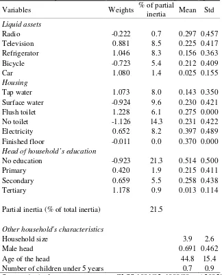
Results from multiple correspondence analysis for the pooled data set are presented
in Table 1. Analysis considers liquid assets as well as housing and education variables.
Weights have signs consistent with interpretation of the first component as an asset-poverty
index. The first dimension of the multiple correspondence analysis explains 21.5% of total
inertia. Variables such as having no toilet, having access to electricity or being not educated
have the largest contribution to inertia (14.3%, 8.2% and 21.3% of partial inertia
respectively). Table 1 also provides means and standard errors for the analysis, on the
various variables used for the asset index as well as on household size, head of household's
gender and age, and the number of children under five years old in the household. For
instance, average household size is 3.9 in Ghana and 39.7% of household have access to
electricity; 51.4% of head of households have no education.
Figure 1 presents the density function of household per capita asset index. This
indicator is normalized to be bounded by 1 and 100. In comparison with the distribution of
per capita household consumption expenditures, per capita household asset index appears to
be more concentrated on the lower tail of the distribution, as it is also the case for per capita
household income. Assets inequality and income inequality thus appear to be more
Taking the analysis one step further, Table 2 presents the Spearman rank correlation
between welfare indicators and shows that per capita household consumption is more
correlated to per capita asset index than to per capita household income. These results are
comparable to those obtained, for instance, by Sahn and Stifel (2003). Furthermore, the
correlation between per capita asset index and other indicators appear to be higher in survey
year 2005/06 than in 1991/92.
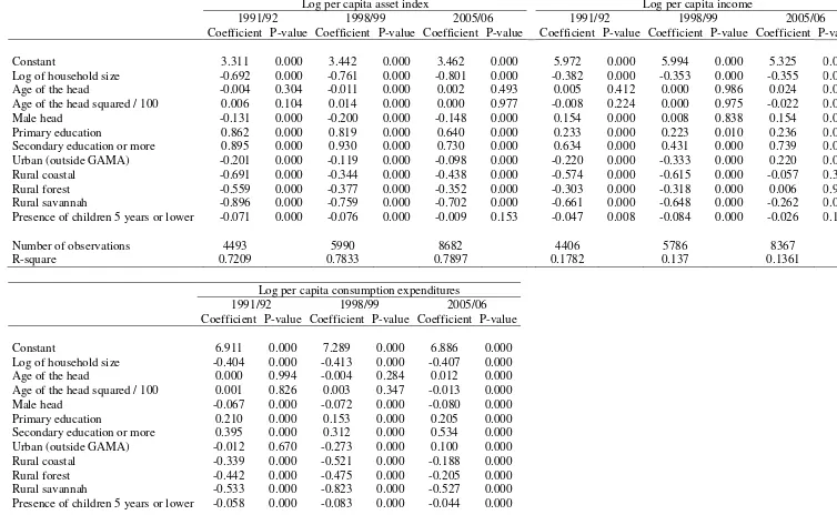
3.2.Estimates
Our estimates of the vulnerability index follow the different steps recalled in the
methodology section. Table 3 presents the first-stage household-level regressions of the
three welfare indicators (household per capita asset index, income and consumption) on
various household’s characteristics such as household size, household head age, gender and
education, and household location. When comparing the different regressions, it appears
that coefficient estimates have the same signs and are rather stable over the three survey
years 1991/92, 1998/99 and 2005/06. While the R-squared is high for the per capita asset
index (around 0.7-0.8), it is rather low for per capita income (around 0.1-0.2); it is
intermediate at about 0.4 for per capita consumption expenditures. One explanation for
such discrepancies is that large measurement errors generally occur when considering
income data. It seems that this is particularly true of GLSS data.
One step further, we propose to measure vulnerability as expected poverty. So, in
order to have a look at the dynamic of the welfare indicators, we regroup households from
the GLSS into cells: households whose heads have the same date of birth (we define
five-year cohorts), the same level of education (no education, primary and secondary and more)
and live in the same region (greater Accra metropolitan area, other urban, rural coastal,
rural forest and rural savannah) are regrouped into the same cells. After regrouping some
low-sized cells,20 166 cells were constituted with the three GLSS surveys, with an average
As described earlier in the methodology section, we calculate for each cell the
variance of the residuals of the first-stage household-level regression. We then regress the
residual variance on cohort dummies (created by crossing household head date of birth,
education and location dummies) and a polynomial function of age (generally of two
degrees or more if statistically significant). From the age profile of the residual variance,
we calculate the slope which is an estimate of the variance of asset, consumption or
income. Note that this slope should necessary be positive (i.e. the amplitude of shocks
grows with age) since the estimated variance should always be positive. This is generally
the case. However, when it is not, contiguous cells have been regrouped for the estimates.
Finally, once the variance of shocks is estimated for each cohort then the last estimation
step consists in drawing values of shocks within the standard normal distribution and
estimating the household vulnerability index using coefficient estimates.
Table 4 presents the percentage of vulnerable households estimated for four poverty
thresholds corresponding to the 25th, 50th, 75th and 90th percentiles of the distribution in
the last available survey and two vulnerability thresholds, 0.5 and 0.29. People are thus
considered as vulnerable when they are more likely to fall into poverty in any period over
two consecutive periods than to not be poor, that is (1–P)2≤0.5, where P is the probability
to fall below the poverty line. So, previous condition can be rewritten as P≥0.29. Instead, a
stricter condition is that people are considered as vulnerable when they are more likely to
fall into poverty than to not be poor in the next period that is P≥0.5. Both vulnerability
thresholds are used in our analysis.
Table 4 shows, for instance, that households in survey year 2005/06 with a poverty
threshold corresponding to the 25th percentile and a vulnerability threshold of 0.5 are
26.9% to be vulnerable to asset-poverty, 29.7% are vulnerable to consumption-poverty and
32.6% are vulnerable to income-poverty. In general, we obtain from our estimates that the
fraction of vulnerable households is higher than the poverty rate. However, in many cases
this gap is larger for income-poverty than for both consumption-poverty and asset-poverty.
These results are consistent with our theoretical framework according to which
households may rather smooth their assets over time instead of smoothing consumption or
income. Consequently, expected asset-poverty underestimates expected
consumption-poverty. The difference between both is however not very large. Table 5 shows that
expected asset-poverty is a better proxy for expected consumption-poverty than is expected
income-poverty. Indeed, Spearman rank correlation is higher between expected
asset-poverty and expected consumption-asset-poverty than it is between expected income-asset-poverty and
expected consumption-poverty, except for survey years 1998/99 and 2005/06 with poverty
threshold of 90%. Furthermore, correlations are of the same order of magnitude as those in
Table 2.
4. CROSS-COUNTRY ANALYSIS USING THE DEMOGRAPHIC HEALTH SURVEYS
4.1.Data
To implement the methodology, we have selected 9 sub-Saharan African countries
with at least 3 standard Demographic Health Surveys (DHS) available (Burkina-Faso,
Ghana, Kenya, Madagascar, Niger, Tanzania, Uganda and Zambia) plus Haiti, a little island
in the Caribbean which is regularly hit by shocks. (See the list of countries in Table 6.) For
our purposes, the DHS have two important characteristics. First, they are conducted in
single rounds on nationally representative samples of around 10,000 households on average
in each survey, with a minimum of about 8,000 households in Niger and a maximum of
about 18,000 households in Madagascar. Large sample sizes is an important feature of the
data since building cells over a large number of households reduces measurement error as
well as bias in estimators based on pseudo-panel data. Second, although survey designs are
not entirely uniform, they are reasonably comparable over time and across countries. This
also proves to be an important feature for our estimates.
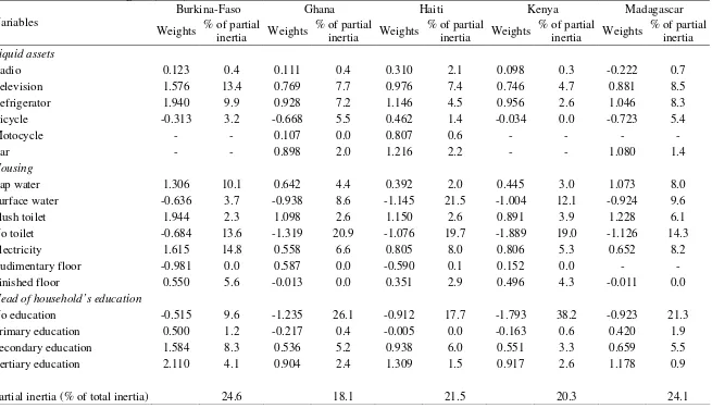
Table 7 presents asset index weights and contribution to inertia of the first
assets (radio, television, refrigerator, bicycle, motorcycle, car), housing characteristics (tap
water, surface water, flush toilet, no toilet, electricity, rudimentary floor, finished floor) and
head of household’s education (no education, primary education, secondary education and
tertiary education). Several items are not available in some countries: motorcycle and car in
Burkina-Faso and Kenya; motorcycle and rudimentary floor in Madagascar and
rudimentary floor in Niger and Uganda. However, these items generally contribute to a
relatively low percentage of inertia. We thus choose to keep them all when available for the
analysis.
Results from multiple correspondence analysis are presented for each country
separately after having pooled the data over the survey periods. Weights have signs
consistent with interpretation of the first component as an asset-poverty index and weights
are generally comparable between countries. However, variables contributions to inertia
vary across countries. For instance, the contribution of having no education appears to be
particularly high (26.1% in Ghana, 17.7% in Haiti, 38.2% in Kenya, 21.3% in Madagascar,
57.6% in Rwanda, 41.4% in Tanzania, 33.3% in Uganda, 22.2% in Zambia), except in
Burkina-Faso (9.6%) and Niger (11.7%). Having no toilet also contributes in a large extent
to inertia (except in Rwanda). Having access to surface water contributes to 21.5% of
inertia in Haiti and 12.1% in Kenya. Owning a television and having access to electricity
contribute to, respectively, 13.4% and 14.8% of inertia in Burkina-Faso. Other items
contribute to less than 10% of inertia.
Table 8 provides descriptive statistics on the main variables for the analysis.
Differences exist between countries. Having no toilets is more frequent in Niger (81.9%),
Burkina-Faso (71.2%) and, to a lesser extent, Madagascar (49.3%) than in other countries.
Countries also differ in terms of tap water access (low access rates, that is lower than 10%,
in Burkina-Faso, Madagascar, Uganda), in terms of electricity access (low access rates in
Burkina-Faso, Niger, Rwanda, Tanzania and Uganda) and in terms of head education
(83.4% have no education in Burkina-Faso and 87.8% in Niger ). Household size is higher
Kenya (23.6%), Madagascar (18.7%), Niger (17.0%), Rwanda (12.3%), Tanzania (24.9%)
and Uganda (14.7%).
4.2.Urban-Rural Comparisons
Several studies have outlined the differences between rural and urban areas in terms
of living standards in Africa.21 For instance, Sahn and Stifel (2003) provide evidence of
large and persistent poverty gap between rural and urban areas using several African DHS.
Yet, for years development economists and policy makers have advocated for the
promotion of rural-focused and agricultural policies to support growth and reduce poverty
and vulnerability. Furthermore, urbanisation trends should have increased inequalities in
urban areas. Consequently, poverty and vulnerability gaps should have decreased over time.
Furthermore, rural-urban differentials in terms of poverty and vulnerability should also vary
across countries due to sectoral specifities or because economies have reached different
stages of urbanisation.
In order to assess the poverty and vulnerability gaps between rural and urban areas
in sub-Saharan African countries, we apply the different steps of our methodology to the
DHS. First, pseudo-panels are built. Table 9 presents the number of cells and cells size
constituted from the data. Mean average size ranges between 111.6 households in Zambia
(with a minimum of 20 households and a maximum of 984 households) and 167.0 in
Rwanda (with a minimum of 20 households and a maximum of 1584 households). The
number of cells ranges from 133 in Burkina-Faso to 254 in Ghana.
Second, log per capita asset index has been regressed on variables presented in
Table 8 (log of household size, age of the head and its square, education and gender of the
head, location and the presence of children under 5 years old). Residuals are estimated from
these regressions. As a result of step 3 and step 4 of the methodology, the percentage of
vulnerable households is estimated and presented in Table 10. In all the countries, urban
vulnerability appears to be higher than rural vulnerability. The gap is higher in
Finally, joint distributions of present wealth and expected future wealth can be
compared using stochastic tests of welfare dominance as presented in the methodology
section. To do so, we estimate bi-dimensional dominance surface for urban and rural areas
using both the present asset index and the simulated (or future) asset index. Dominance
surfaces are calculated for various thresholds corresponding to the deciles of both present
and simulated future asset distributions. Then, t-statistics are computed for the difference
between urban and rural areas. Differences are estimated at dominance orders (1,1) and
(2,2). The results confirm that urban areas unambiguously dominate rural areas in terms of
present wealth and expected future wealth in all the country considered. The results are
statistically significant at less than 1 percent level for all thresholds and all countries.
Results are presented for Madagascar in Table 11. Table 11 also reports differences in
poverty incidence. All reported differences are statistically significant at less than 1 percent
level.
5. CONCLUSION
In this paper, we present a simple and intuitively appealing framework to assess
vulnerability to asset-poverty. The approach draws on a model of asset smoothing
behaviour that is based on the idea that households will prefer to keep their assets
unchanged when facing adverse shocks on them. We use age-cohort decomposition
techniques focusing on second-order moments in order to identify and estimate the variance
of shocks on assets. Estimates are used to simulate expected asset-poverty. This approach
can be applied to repeated cross-section data that are available in many developing
countries.
Applying this methodology to Ghana Living Standard Surveys, we find that
expected asset-poverty slightly underestimates expected consumption-poverty.
Furthermore, expected asset-poverty appears to be a better proxy for expected
to assess vulnerability to asset-poverty. Cross-country comparisons show a clear
vulnerability gap between urban and rural areas. What is more, joint distributions of present
wealth and expected future wealth are compared using stochastic tests of welfare
dominance. Welfare differences between urban and rural areas appear large, robust and
statistically significant for all the country considered. Consequently, in these countries,
policies and programs should aim at increasing or securing assets of the most vulnerable
NOTES
1 See, among others, Glewwe and Hall (1998), Pritchett et al. (2000), Chaudhuri et al.
(2002), Chaudhuri (2003), Ligon and Schechter (2003), Christiaensen and Subbarao (2005), Calvo and Dercon (2005), Calvo (2008), Günther and Harttgen (2009).
2
See, for instance, the literature review by Hoddinott and Quisumbing (2003).
3
What is more, we have to choose a probability threshold under which people should be considered vulnerable. An intuitive threshold is when the probability of being poor in the future exceeds 50%: people should be considered vulnerable in this case since they are more likely to fall into poverty than to not be poor in the future (Pritchett et al., 2000).
4
See, for instance, Sahn and Stifel (2000), Filmer and Pritchett (2001), Sahn and Stifel (2003), Booysen et al. (2008).
5 This list of assets is not exhaustive and could be completed following Moser (1998)’s
asset-based approach. In her asset vulnerability framework, Moser (1998) identifies several categories of assets and illustrates how portfolio management affects vulnerability. Asset management includes: labor (e.g., the number of earners in the family and their income level), human capital (education and health), productive assets (such as housing in urban areas or cattle in rural areas), household relations and social capital.
6
Sahn and Stifel (2003) show that an asset index obtained from a factor analysis on household assets using multipurpose surveys from several developing countries is a valid predictor of child health and nutrition and, thus, long term poverty.
7
I thank a referee for suggesting me this point.
8 See, among others, Rosenzweig and Wolpin (1993), Morduch (1995), Fafchamps et al.
(1998), Kazianga and Udry (2006), and Hoddinott (2006).
9
Zimmerman and Carter (2003) and Carter and Barrett (2006), among others, have analyzed the existence of poverty traps when households are involved in various asset accumulation dynamics.
10
Note that if households are able to diversify their portfolio of assets into risky and safe assets, then in presence of credit constraints they will choose to lower the proportion of risky assets held in order to smooth income over time (Morduch, 1994).
11
The empirical evidence concerning the existence of such asset-poverty traps and thresholds are mixed with some authors finding evidence of its existence: see, for instance, Lybbert et al. (2004), Adato et al. (2006), Barret et al. (2006) or Carter et al. (2007). Carter and May (1999, 2001) also provide evidence of poverty traps although they are differently theoretically grounded.
12 Bourguignon and Goh (2004) proposed a similar method for assessing vulnerability to
poverty, although relying on earning dynamics.
13
A cohort is typically defined by the year of birth, education level and location.
14
As exposed by Verbeek and Nijman (1992), the bias in the standard within estimator based on pseudo panel data is decreasing with the number of individuals in each cell, more than with the number of cells. However, Verbeek (2008) notes that there is no general rule to judge whether cell size is large enough. Deaton (1985) also suggests that measurement error decreases as a function of the size of the cells.
15
17
Note that estimates were replicated using a more restrictive definition of the asset index for which only liquid assets were included in the analysis; but no sizeable differences were obtained for the evaluation of vulnerability to poverty from these estimates.
18
See Benzécri (1973) or, more recently, Asselin (2009).
19
Alternatively, Sahn and Stifel (2000) used factor analysis, and Filmer and Pritchett (2001) used principal component analysis to measure their asset index. In reference to these methodologies, multiple correspondence analysis can be viewed as a principal component analysis applied to a contingency table with the chi2-metric being used on the row/column profiles, instead of the usual Euclidean metric. Multiple correspondence analysis provides information similar in nature to those produced by factor analysis and is less restrictive than principal component analysis.
20 Note that cells with less than 20 households have been regrouped in order to minimize
measurement error.
21
REFERENCES
Alderman, H., Hoddinott, J., and B. Kinsey (2002), “Long term consequences of early childhood malnutrition,” mimeo, FCND, International Food Policy Research Institute, Washington D.C.
Antman, F., and D. J. McKenzie (2007), “Poverty traps and nonlinear income dynamics with measurement error and individual heterogeneity,” Journal of Development Studies, 43(6), 1057-1083.
Asselin, L-M. (2009), Analysis of multidimensional poverty: Theory and case studies. Springer.
Behrman, J., Alderman, H., and J. Hoddinott (2004), “Hunger and malnutrition,” in Global Crises, Global Solutions, B. Lomborg (ed.). Cambridge (UK): Cambridge University Press.
Benzécri, J.P. (1973), L’analyse des données 2 : L’analyse des correspondances. Paris: Dunod.
Booysen F., van der Berg, S., von Maltitz, M., and G. du Rand (2008), “Using an asset index to assess trends in poverty in seven sub-Saharan African countries,” World Development, 36(6), 1113-1130.
Bourguignon, F., and C. Goh (2004), “Trade and labor vulnerability in Indonesia, Republic of Korea, and Thailand,” in Kharas, H., and K. Krumm (eds), East Asia integrates: a trade policy agenda for shared growth. World Bank and Oxford University Press, Washington DC.
Calvo, C. (2008), “Vulnerability to multidimensional poverty: Peru, 1998–2002”, World Development, 36(6), 1011–1020.
Calvo, C., and S. Dercon (2005), “Measuring individual vulnerability,” Oxford Economics Discussion Paper, 229.
Carroll, C. (1992), “The buffer-stock theory of saving: Some macroeconomic evidence,” Brookings Papers on Economic Activity, 23(2), 61-156.
Carter, M. R., and C. B. Barrett (2006), “The economics of poverty traps and persistent poverty: An asset-based approach,” Journal of Development Studies, 42(2), 178–199. Chaudhuri, S. (2003), “Assessing vulnerability to poverty: concepts, empirical methods and
illustrative examples,” mimeo, Department of economics, Columbia University
Chaudhuri S., Jalan, J., and A. Suryahadi (2002), “Assessing household vulnerability to poverty from cross-sectional data: a methodology and estimates from Indonesia,” Discussion Paper 0102-02, Department of Economics, Columbia University.
Christiaensen, L., and K. Subbarao (2005), “Towards an understanding of vulnerability in rural Kenya,” Journal of African Economies, 14(4), 520-558.
Coulombe, H., and Q. Wodon (2007), “Poverty, livelihoods, and access to basic services in Ghana,” The World Bank, Washington DC.
Deaton, A., and C. Paxson (1994), “Intertemporal choice and inequality,” Journal of Political Economy, 102(3), 437-467.
De Ferranti, D., Perry, G. E., and L. Serven (2000), Securing our Future in a Global Economy. World Bank, Washington DC.
Dercon, S. (1998) Wealth, risk and activity choice: cattle in Western Tanzania. Journal of
Development Economics, 55, 1-42.
Dercon, S. and Krishnan, P. (2003) Risk sharing and public transfers. Economic Journal,
113(486), C86-C94.
Duclos, J.-Y.. Sahn, D. E. and S. D. Younger (2011), “Partial multidimensional inequality orderings,” Journal of Public Economics, 95(3-4), 225-238.
Fafchamps, M., Udry, C., and K. Czukas (1998), “Drought and saving in West Africa: Are livestock a buffer stock?” Journal of Development Economics, 55(2), 273-305.
Filmer, D., and L. H. Pritchett (2001), “Estimating wealth effects without expenditure data—or tears: An application to educational enrollments in states of India,” Demography, 38(1), 115-132.
Glewwe, P., and G. Hall (1998), “Are some groups more vulnerable to macroeconomic shocks than others? Hypothesis tests based on panel data from Peru,” Journal of Development Economics, 56(1), 181-206.
Hoddinott, J. (2006), “Shocks and their consequences across and within households in rural Zimbabwe,” Journal of Development Studies, 42(2), 301-321.
Hoddinott, J., and A. Quisumbing (2003), “Methods for microeconometric risk and vulnerability assessment,” Social Protection Discussion Paper Series 0324.
Kazianga, H., and C. Udry (2006), “Consumption smoothing? Livestock, insurance and drought in rural Burkina Faso,” Journal of Development Economics, 79(2), 413-446. Ligon, E., and L. Schechter (2003), “Measuring vulnerability,” Economic Journal,
113(486), 95-102.
McPeak, J. (2004), “Contrasting income shocks with asset shocks: livestock sales in northern Kenya,” Oxford Economic Papers, 56(2), 263-284.
Morduch, J. (1994), “Poverty and vulnerability”, American Economic Review, Papers and Proceedings, 84(2), 221-225.
Morduch, J. (1995), “Income smoothing and consumption smoothing”, Journal of Economic Perspectives, 9(3), 103-114.
Morduch, J., and G. Kamanou (2004), “Measuring vulnerability to poverty,” in Insurance Against Poverty, S. Dercon (ed.). Oxford University Press.
Moser, C. (1998), “The asset vulnerability framework: Reassessing urban poverty reduction strategies,” World Development, 26(1), 1–19.
Pritchett, L., Suryahadi, A., and S. Sumarto (2000), “Quantifying vulnerability to poverty: A proposed measure, applied to Indonesia,” World Bank Social Monitoring and Early Response Unit.
Rosenzweig, M., and H. Wolpin (1993), “Credit market constraints, consumption smoothing, and the accumulation of durable production assets in low-income countries: investment in bullocks in India,” Journal of Political Economy, 101(2), 223-244.
Sahn, D. E., and D. C. Stifel (2000), “Poverty comparisons over time and across countries in Africa,” World Development, 28(12), 2123–2155.
Sahn, D. E., and D. C. Stifel (2003), “Urban–rural inequality in living standards in Africa,” Journal of African Economies, 12(4), 564–597.
Verbeek, M., and T. Nijman (1992), “Can cohort data be treated as genuine panel data?,” Empirical Economics, 17(1), 9–23.
Verbeek, M. (2008), “Pseudo-panels and repeated cross-sections,” Advanced Studies in
Theoretical and Applied Econometrics, 46(2), 369-383.
World Bank (2000), World Development Report 2000/2001: Attacking poverty. New York: The World Bank and Oxford University Press.
World Bank (2009), World Development Report 2010: Climate change. The World Bank, Washington DC.
Table 1. Descriptive statistics and asset index weights for pooled data (GLSS)
Variables Weights % of partial
inertia Mean Std
Liquid assets
Radio -0.222 0.7 0.297 0.457 Television 0.881 8.5 0.225 0.417 Refrigerator 1.046 8.3 0.156 0.363 Bicycle -0.723 5.4 0.212 0.409 Car 1.080 1.4 0.025 0.155
Housing
Tap water 1.073 8.0 0.143 0.350 Surface water -0.924 9.6 0.230 0.421 Flush toilet 1.228 6.1 0.275 0.000 No toilet -1.126 14.3 0.231 0.422 Electricity 0.652 8.2 0.397 0.489 Finished floor -0.011 0.0 0.370 0.000
Head of household’s education
No education -0.923 21.3 0.514 0.500 Primary 0.420 1.9 0.215 0.411 Secondary 0.659 5.5 0.258 0.438 Tertiary 1.178 0.9 0.013 0.114
Partial inertia (% of total inertia) 21.5
Other household's characteristics
Household size 3.9 2.6
Male head 0.691 0.462
Age of the head 44.8 15.4 Number of children under 5 years 0.7 0.9
Figure 1. Kernel density estimates of welfare indicators (GLSS) 0 .0 2 .0 4 .0 6 D e n s it y
0 20 40 60 80 100
Overall (Gini=0.4811) 1991/1992 (Gini=0.4794) 1995/1996 (Gini=0.4592) 2005/2006 (Gini=0.4905)
kernel = epanechnikov, bandwidth = 1.7892
Per Capita Asset Index
0 .0 0 0 5 .0 0 1 .0 0 1 5 .0 0 2 .0 0 2 5 D e n s it y
0 200 400 600 800 1000
Overall (Gini=0.5790) 1991/1992 (Gini=0.5329) 1997/1998 (Gini=0.5526) 2005/2006 (Gini=0.5965)
kernel = epanechnikov, bandwidth = 32.6141
Per Capita Income
0 .0 0 0 5 .0 0 1 .0 0 1 5 .0 0 2 D e n s it y
0 200 400 600 800 1000
Overall (Gini=0.4271) 1991/1992 (Gini=0.3972) 1997/1998 (Gini=0.4033) 2005/2006 (Gini=0.4350)
kernel = epanechnikov, bandwidth = 32.6739
Per Capita Consumption
Source: Author’s computations using GLSS 1991/92, 1998/99 and 2005/06. Note: Consumption and income are expressed in 2006 US$.
Table 2. Spearman rank correlations between consumption expenditures and alternative measures of welfare (GLSS)
Survey year Asset index Income 1991/92 0.62 0.53 1998/99 0.64 0.58 2005/06 0.68 0.58
Table 3. First-stage household-level regressions (GLSS)
Log per capita asset index Log per capita income
1991/92 1998/99 2005/06 1991/92 1998/99 2005/06 Coefficient P-value Coefficient P-value Coefficient P-value Coefficient P-value Coefficient P-value Coefficient P-val
Constant 3.311 0.000 3.442 0.000 3.462 0.000 5.972 0.000 5.994 0.000 5.325 0.00 Log of household size -0.692 0.000 -0.761 0.000 -0.801 0.000 -0.382 0.000 -0.353 0.000 -0.355 0.00 Age of the head -0.004 0.304 -0.011 0.000 0.002 0.493 0.005 0.412 0.000 0.986 0.024 0.00 Age of the head squared / 100 0.006 0.104 0.014 0.000 0.000 0.977 -0.008 0.224 0.000 0.975 -0.022 0.00 Male head -0.131 0.000 -0.200 0.000 -0.148 0.000 0.154 0.000 0.008 0.838 0.154 0.00 Primary education 0.862 0.000 0.819 0.000 0.640 0.000 0.233 0.000 0.223 0.010 0.236 0.00 Secondary education or more 0.895 0.000 0.930 0.000 0.730 0.000 0.634 0.000 0.431 0.000 0.739 0.00 Urban (outside GAMA) -0.201 0.000 -0.119 0.000 -0.098 0.000 -0.220 0.000 -0.333 0.000 0.220 0.00 Rural coastal -0.691 0.000 -0.344 0.000 -0.438 0.000 -0.574 0.000 -0.615 0.000 -0.057 0.31 Rural forest -0.559 0.000 -0.377 0.000 -0.352 0.000 -0.303 0.000 -0.318 0.000 0.006 0.90 Rural savannah -0.896 0.000 -0.759 0.000 -0.702 0.000 -0.661 0.000 -0.648 0.000 -0.262 0.00 Presence of children 5 years or lower -0.071 0.000 -0.076 0.000 -0.009 0.153 -0.047 0.008 -0.084 0.000 -0.026 0.14
Number of observations 4493 5990 8682 4406 5786 8367
R-square 0.7209 0.7833 0.7897 0.1782 0.137 0.1361
Log per capita consumption expenditures 1991/92 1998/99 2005/06 Coefficient P-value Coefficient P-value Coefficient P-value
Number of observations 4493 5990 8682 R-square 0.4155 0.4243 0.4363 Source: Author’s computations using GLSS 1991/92, 1998/99 and 2005/06.
Table 4. Percentage of vulnerable households (GLSS)
1991/92 1998/99 2005/2006
Vulnerability threshold
Poverty
threshold Asset index Consumption Income Asset index Consumption Income Asset index Consumption Income 29% 25% 25.6 27.2 28.9 36.0 35.6 37.9 26.9 29.7 32.6
50% 50.5 51.8 54.2 56.8 57.9 59.8 51.8 54.0 56.5 75% 75.9 76.1 78.7 78.8 79.9 80.7 76.0 77.1 79.0 90% 90.2 90.6 91.1 91.6 92.2 92.6 90.9 91.0 91.6 50% 25% 25.2 25.6 26.9 35.7 34.2 36.4 26.6 28.4 30.9 50% 50.1 50.0 51.5 56.4 56.5 57.8 51.4 52.8 54.2 75% 75.5 75.0 75.7 78.5 79.0 78.6 75.6 76.4 77.1 90% 89.7 90.2 90.1 91.4 91.8 91.5 90.6 90.5 90.6 Source: Author’s computations using GLSS 1991/92, 1998/99 and 2005/06.
[image:31.792.51.491.319.403.2]Note: Welfare indices are expressed per capita.
Table 5. Spearman rank correlations between expected consumption poverty and alternative expected poverty indices (GLSS)
1991/92 1998/99 2005/06
Poverty
threshold Asset index Income Asset index Income Asset index Income 25% 0.46 0.42 0.55 0.46 0.59 0.51 50% 0.53 0.48 0.57 0.53 0.60 0.54 75% 0.52 0.46 0.49 0.48 0.53 0.49 90% 0.45 0.39 0.38 0.41 0.38 0.40 Source: Author’s computations using GLSS 1991/92, 1998/99 and 2005/06.
Table 6. List of DHS countries
Country name Survey years
Burkina-Faso (1993, 1998-99, 2003)
Ghana (1988, 1993, 1998, 2003, 2008) Haiti (1994-95, 2000, 2005-06) Kenya (1989, 1993, 1998, 2003) Madagascar (1992, 1997, 2003-04, 2008-09) Niger (1992, 1998, 2006)
Rwanda (1992, 2000, 2005)
Tanzania (1991-92, 1996, 1999, 2004-05) Zambia (1992, 1996, 2001-02, 2007)
Table 7. Asset index weights (DHS)
Burkina-Faso Ghana Haiti Kenya Madagascar Variables
Weights % of partial
inertia Weights
% of partial
inertia Weights
% of partial
inertia Weights
% of partial
inertia Weights
% of partial inertia
Liquid assets
Radio 0.123 0.4 0.111 0.4 0.310 2.1 0.098 0.3 -0.222 0.7 Television 1.576 13.4 0.769 7.7 0.976 7.4 0.746 4.7 0.881 8.5 Refrigerator 1.940 9.9 0.928 7.2 1.146 4.5 0.956 2.6 1.046 8.3 Bicycle -0.313 3.2 -0.668 5.5 0.462 1.4 -0.034 0.0 -0.723 5.4
Motocycle - - 0.107 0.0 0.807 0.6 - - - -
Car - - 0.898 2.0 1.216 2.2 - - 1.080 1.4
Housing
Tap water 1.306 10.1 0.642 4.4 0.392 2.0 0.445 3.0 1.073 8.0 Surface water -0.636 3.7 -0.938 8.6 -1.145 21.5 -1.004 12.1 -0.924 9.6 Flush toilet 1.944 2.3 1.098 2.6 1.150 2.6 0.891 3.9 1.228 6.1 No toilet -0.684 13.6 -1.319 20.9 -1.076 19.7 -1.889 19.0 -1.126 14.3 Electricity 1.615 14.8 0.558 6.6 0.805 8.0 0.806 5.3 0.652 8.2 Rudimentary floor -0.981 0.0 0.587 0.0 -0.590 0.1 0.152 0.0 - - Finished floor 0.550 5.6 -0.013 0.0 0.351 2.9 0.496 4.3 -0.011 0.0
Head of household’s education
No education -0.515 9.6 -1.235 26.1 -0.912 17.7 -1.793 38.2 -0.923 21.3 Primary education 0.500 1.2 -0.217 0.4 -0.005 0.0 -0.163 0.6 0.420 1.9 Secondary education 1.584 8.3 0.536 5.2 0.938 6.0 0.551 3.3 0.659 5.5 Tertiary education 2.110 4.1 0.904 2.4 1.309 1.5 0.917 2.6 1.178 0.9
Niger Rwanda Tanzania Zambia Variables
Weights % of partial
inertia Weights
% of partial
inertia Weights
% of partial
inertia Weights
% of partial inertia
Liquid assets
Radio 0.150 0.5 0.236 1.5 0.150 0.7 0.221 0.9 Television 1.421 9.9 1.100 2.6 1.236 4.4 0.876 5.2 Refrigerator 1.594 6.8 1.103 1.9 1.317 3.9 1.053 4.2 Bicycle 0.505 1.1 0.441 1.2 -0.058 0.1 -0.220 0.6 Motocycle 1.058 3.4 1.200 1.7 1.240 2.3 1.044 0.6 Car 1.446 3.9 1.246 2.3 1.369 3.0 1.034 1.6
Housing
Tap water 0.792 5.7 0.497 1.6 0.449 2.7 0.753 5.7 Surface water -0.800 8.2 -0.669 6.0 -0.914 9.2 -0.862 9.1 Flush toilet 1.647 2.3 1.094 0.8 1.175 1.9 1.001 5.3 No toilet -0.752 18.5 -0.994 3.1 -1.122 11.5 -1.221 19.2 Electricity 1.288 10.4 0.938 4.2 1.027 7.0 0.977 6.5 Rudimentary floor - - -0.579 0.0 -0.998 0.0 0.739 0.0 Finished floor 0.977 9.8 0.661 4.5 0.637 6.1 0.624 5.9
Head of household’s education
No education -0.552 11.7 -1.505 57.6 -1.512 41.4 -1.690 22.2 Primary education 0.458 0.8 0.403 5.1 0.144 0.7 -0.566 6.8 Secondary education 1.276 4.3 0.903 4.7 0.907 3.7 0.553 3.4 Tertiary education 1.720 2.9 1.108 1.1 1.239 1.5 1.017 2.8
Table 8. Descriptive statistics (DHS)
Burkina-Faso Ghana Haiti Kenya Madagascar Niger Rwanda Tanzania Zambia Variables
Mean Std Mean Std Mean Std Mean Std Mean Std Mean Std Mean Std Mean Std Mean Std
Liquid assets
Radio 0.583 0.556 0.628 0.540 0.513 0.505 0.662 0.503 0.526 0.517 0.413 0.556 0.389 0.509 0.494 0.509 0.459 0.512 Television 0.097 0.420 0.297 0.511 0.226 0.422 0.181 0.484 0.128 0.351 0.061 0.373 0.025 0.290 0.042 0.263 0.180 0.416 Refrigerator 0.049 0.362 0.194 0.463 0.093 0.294 0.051 0.322 0.028 0.173 0.032 0.291 0.016 0.225 0.032 0.242 0.098 0.383 Bicycle 0.755 0.490 0.220 0.452 0.145 0.355 0.267 0.463 0.155 0.384 0.073 0.302 0.095 0.390 0.355 0.529 0.291 0.471 Motocycle - - 0.031 0.247 0.017 0.131 - - - - 0.043 0.264 0.017 0.330 0.018 0.302 0.013 0.275 Car - - 0.055 0.304 0.040 0.198 - - 0.022 0.205 0.026 0.293 0.019 0.339 0.024 0.321 0.039 0.327
Housing
Tap water 0.087 0.282 0.238 0.433 0.325 0.473 0.306 0.461 0.072 0.257 0.124 0.333 0.080 0.272 0.196 0.400 0.269 0.441 Surface water 0.215 0.410 0.201 0.407 0.342 0.479 0.269 0.443 0.343 0.473 0.325 0.473 0.224 0.418 0.223 0.419 0.276 0.444 Flush Toilet 0.013 0.114 0.048 0.217 0.054 0.228 0.097 0.296 0.011 0.106 0.008 0.090 0.008 0.090 0.020 0.139 0.150 0.355 No Toilet 0.712 0.453 0.198 0.405 0.378 0.490 0.117 0.321 0.493 0.498 0.819 0.389 0.051 0.220 0.130 0.338 0.287 0.450 Electricity 0.097 0.392 0.490 0.537 0.333 0.476 0.167 0.412 0.156 0.367 0.077 0.341 0.050 0.272 0.108 0.395 0.182 0.399 Rudimentary Floor 0.000 0.013 0.002 0.040 0.005 0.072 0.005 0.073 - - - - 0.000 0.015 0.001 0.026 0.002 0.041 Finished Floor 0.341 0.474 0.861 0.352 0.560 0.501 0.371 0.483 0.234 0.422 0.130 0.340 0.125 0.332 0.237 0.428 0.391 0.485
Head of household’s education
No education 0.834 0.372 0.326 0.477 0.476 0.504 0.236 0.424 0.268 0.441 0.878 0.331 0.418 0.494 0.311 0.466 0.168 0.372 Primary Education 0.091 0.288 0.191 0.400 0.333 0.476 0.466 0.499 0.483 0.498 0.071 0.259 0.497 0.501 0.613 0.490 0.488 0.497 Secondary Education 0.058 0.233 0.417 0.501 0.167 0.377 0.237 0.425 0.218 0.412 0.037 0.192 0.075 0.264 0.055 0.229 0.273 0.443 Tertiary Education 0.017 0.128 0.064 0.249 0.024 0.154 0.060 0.238 0.029 0.168 0.011 0.107 0.009 0.092 0.018 0.133 0.068 0.251
Other household's characteristics
Table 9. Cell sizes (DHS)
Mean Minimum Maximum Number of cells