Munich Personal RePEc Archive
Intergenerational earnings and income
mobility in Spain
Cervini-Plá, María
Universitat de Girona
16 November 2011
Online at
https://mpra.ub.uni-muenchen.de/34942/
Intergenerational earnings and income mobility in
Spain
Mar´ıa Cervini-Pl´
a
∗November 16, 2011
Abstract
This paper contributes to the large number of studies on intergenerational earnings and income mobility by providing new evidence for Spain. Since there are no Spanish surveys covering long-term information on both children and their fathers’ income or earnings, we deal with this selection problem using the two-sample two-stage least squares estimator. We find that intergenerational mobility in Spain is similar to France, lower than in the Nordic countries and Britain and higher than in Italy and the United States. Furthermore, we use the Chadwick and Solon (2002) approach to explore the intergenerational mobility in the case of daughters overcoming employment selection, and we find similar results by gender.
Keywords: Intergenerational earnings and income mobility, two sample two stage least squares estimator, Spain.
JEL classification: D31, J31, J62.
1
Introduction
Intergenerational mobility refers to the association between socioeconomic
achieve-ments of parents and those of their children. If we believe that equal opportunity is
a desirable characteristic of society, a high degree of intergenerational mobility is an
important indicator of the health and success of society. In this context, the
socioeco-nomic status of children from different families are not predetermined by their parents
and they have equal options to achieve education and higher earnings (Behrman and
Taubman (1990)).
Intergenerational mobility studies usually estimate the correlation between the
socioeconomic status of parents and their offspring. On the one hand, a high
corre-lation would imply that people born in disadvantaged families have a smaller chance
to occupy the highest socioeconomic positions than those born in privileged families.
On the other hand, a zero correlation would imply a high degree of mobility and more
equal opportunities. Sociologists explore the association measures between ordered
categorical variables, such as social and economic class position. Meanwhile the
eco-nomics literature has primarily concentrated on the relationship between parents’ and
their offspring’s permanent incomes or earnings.1 In particular, the standard measure
of intergenerational mobility that economists use is earnings or income elasticity.
In this paper, we contribute to the empirical literature by estimating the earnings
and income mobility for Spain. In general these type of papers estimate the elasticity
only for sons to avoid the typical employment selection of daughters. Therefore,
an-other important contribution of our paper is to explore the intergenerational earnings
mobility for daughters.
The estimation of intergenerational mobility can be biased due to different sample
selection problems. One of these problems arises from the fact that, in a panel, we have
information regarding offspring’s and parents’ earnings when they live together in at
least one wave; however, the probability of observing offspring living with their parents
decreases as the children grow older. Thus, in short panels, it is impossible to follow
children during their adult life.2 This selection problem is particularly important in
1
See Solon (1999), Bj¨orklund and J¨antti (2000), Bowles and Gintis (2002), Erikson and Goldthorpe (2002) for a review.
2
Spain, where we have only short panels, and thus, do not have information on both
children’s and their fathers’ permanent earnings. When we have information regarding
the father, the children are too young to observe their permanent earnings, and when
we have adults, we do not have information about their father’s earnings.
In order to overcome this selection problem, it is possible to estimate
intergen-erational earnings mobility using the two-sample two-stage least squares (TSTSLS)
estimator.3 This method combines information from two separate samples: a sample
of adults (sons and daughters) with observations of their earnings and their parents’
characteristics, and a sample of potential parents with observations on earnings and
the same characteristics. The latter sample is used to estimate an earnings equation
for parents using their characteristics as explanatory variables, while the former is used
to estimate an intergenerational earnings equation by replacing the missing parents’
earnings with its best linear prediction.
When we want to study the intergenerational earnings mobility in the case of
daughters, a second problem that arises is the employment selection, wherein we only
have earnings for adults who are employed. Since the decision to work or not work
is not random, especially in the case of women, estimating intergenerational earnings
mobility only for those who are working gives us biased estimators. To give some
intuitions of what happens in the case of daughters, we deal with this selection problem
following Chadwick and Solon (2002) and using family incomes instead of daughter’s
individual earnings.
Why Spain? The literature on intergenerational earnings mobility has concentrated
on the United States, Canada, and some European countries, including England,
Scan-dinavian countries, Germany, and France. However, there is comparably less evidence
for the intergenerational mobility in southern European countries, probably due to
the lack of long panels. The studies of Mocetti (2007) and Piraino (2007) are two
Nicoletti and Francesconi (2006) analyse intergenerational mobility using an occupational prestige score. They find that the β coefficient (where β represents the elasticity between father’s and off-spring’s occupational prestige scores) is underestimated when they only consider the pairs of children and parent who are cohabiting.
3
exceptions, exploring intergenerational earnings mobility in Italy.
As in other southern European countries, Spain experiences stronger
intergener-ational family bonds compared to other countries outside the region. Indeed after
leaving home, children maintain a close relationship with parents. Therefore, it is
valuable to explore how earnings mobility in Spain compares to other countries, and it
is particularly interesting to compare our results to those obtained by Mocetti (2007)
and Piraino (2007) for Italy.
Intergenerational mobility in Spain has primarily been studied by sociologists. For
example, Caraba˜na (1999) studied occupational mobility. From an economic point
of view, Sanchez-Hugalde (2004) analyses the intergenerational income and education
mobility in Spain using the Family Expenditure Survey (Encuesta de Presupuestos
Familiares) for 1980 and 1990; however, she only estimates the elasticity when children
and their fathers live together. Another recent study about the intergenerational
mobility in Spain is the paper of G¨uell, Mora, and Telmer (2007), in which they study
the information contained in the surnames of the inhabitants of a large Spanish region
as indicative of the degree of intergenerational mobility of an economy. The idea is
that surnames capture family links in a manner that allows them to be used to extract
longitudinal information from census data.
We find an elasticity around 0.40 for sons. When we analyse daughters following
Chadwick and Solon (2002) approach we find nearly the same elasticities as for sons.
By comparing the elasticities obtained in Spain with the results for other countries,
we find that intergenerational mobility in Spain is similar to mobility in France, is
lower than in Nordic countries and Britain, and is higher than in Italy and the United
States.
The rest of the paper is organised as follows. In the next section, we describe
how we implement the two-sample two-stage least squares estimator. In Section 3 we
describe the data source, the selection sample, and the variables used in the empirical
analysis. In Section 4, we report the results, and finally, in Section 5, we offer some
2
Estimation method
2.1
The econometric model
As we explained above, we focus on intergenerational mobility measured by the
in-tergenerational elasticity of children’s earnings (or income) with respect to paternal
earnings (or income). More precisely, we consider the following intergenerational
mo-bility equation:
Wit =α+βWit−1+µit (1)
where Wit is the children’s log earnings (or our economic variable of permanent
income), Wit−1 is the fathers’ log earnings (the economic variable of the previous
generation), α is the intercept term representing the average change in the child’s log
earnings, and µis a random error. The coefficient β is the intergenerational elasticity
of children’s earnings with respect to their father’s earnings, and it is our parameter
of interest.
Let ρ be the correlation between Wit and Wit−1; then β is related to ρ by the
following equation:
β =ρ σWit σWit
−1
(2)
where σ is the standard deviation. In other words, the coefficient is related to the
correlation between children’s and fathers’ log earnings. In particular, the coefficient
β will be exactly equal to ρ when: σWit
−1 =σWit.
On the one hand, when β = 0, sons’ earnings are not determined by their fathers’
earnings. On the other hand, a value of β = 1 represents a situation of complete
immobility; that is, children’s earnings are fully determined by their fathers’
earn-ings. Generally, the coefficient is between these two values. Therefore, to evaluate
adequately if the coefficient is high or low, it is necessary to compare the results to
those found for other countries.
If we had permanent income for successive generations in our sample, we would
directly estimate equation 1 using the ordinary least squares estimator without any
First, most data sets only provide measures of current earnings and fail to provide
measures of individual permanent income. Solon (1992) and Zimmerman (1992) show
that the use of current earnings as a proxy for permanent earnings leads to downward
OLS estimates of β. Different solutions can be implemented to reduce or eliminate
this bias. If we work with panel data, we can calculate an average of current earnings
over several years as a proxy of permanent income. Another possibility lies in using
instrumental variables to estimateβ. In this paper, in the case of the father’s earnings,
we estimate it by using auxiliary variables. Therefore, the estimated earnings is an
average that can be considered as a proxy of the father’s permanent earnings. In the
case of children, we select adult ages as close as possible to the age in which earnings
are similar to permanent income. In particular, Haider and Solon (2006) suggests the
use of offspring around 40 years old.
Second, we also have other selection problems that lead us to inconsistent
estima-tions of β. In the next subsection, we describe the main selection problems that we
face and how we solve them in this paper.
2.2
Two sample two stage least squares estimator
The estimation of intergenerational earnings mobility can frequently be biased due to
different sample selection problems. One of the most important selection problems
we experience in short panels is the fact that we only observe earnings for pairs of
parents and children when they live together in at least one wave of the panel. On
the contrary, we do not have information for sons who never co-reside with their
parents during the panel. This selection problem could lead to a sub-estimation of
the offspring’s earnings, since living in the parental household is either because they
are still students or they do not have enough income to live alone. Thus, they are
not a random sample. In general, this selection problem causes an overestimation
of intergenerational mobility (an underestimation of the elasticity between parents’
earnings and offspring’s earnings).
If the panel is long, we do not have to deal with this selection problem, as it is
easy to observe young children living together with their parents and follow them to
We deal with this selection problem linking two samples and using the TSTSLS
estimator. We use one sample with information on adults and the characteristics
(occupation, education, age) of the fathers when the sons are between 12 and 14 years
old, and another sample with the same paternal characteristics, but also with their
earnings.
The TSTSLS estimator is a computationally easier variant of two-sample
instru-mental variable estimator (2SIV) described by Angrist and Krueger (1992), Arellano
and Meghir (1992), and Ridder and Moffit (2006).4 Concretely, in the two-sample
con-text, unlike the single-sample situation, the IV and 2SLS estimators are numerically
distinct. Inoue and Solon (2010) derive and compare the asymptotic distributions
of the two estimators and find that the commonly used TSTSLS estimator is more
asymptotically efficient than the TSIV estimator because it implicitly corrects for
dif-ferences in the distribution of variables between the two samples. Therefore, they
explain that, although computationally simplicity was the original motive that drew
applied researchers to use the TSTSLS estimator instead of the TSIV estimator, it
turns out that the TSTSLS estimator also is theoretically superior.
Since we do not have information about Wit−1, but do have a set of instrumental
variablesZ ofWit−1, we can estimate equation (1) in two steps. As we have explained
before, we consider two different samples: The first, which we call the main sample,
has data on offspring log earnings, Wit, and characteristics of their fathers, Z, while
the second, which we call the supplemental sample, has information on fathers’ log
earnings, Wt−1, and their age, education, and occupational characteristics, Z. In
the previous studies that estimate intergenerational mobility combining two different
datasets, different variables have been used to impute the missing father’s earnings.5
In the first step, we use the supplemental sample to estimate a log earnings equation
4
For a detailed description of the properties of this estimator, see Arellano and Meghir (1992), Angrist and Krueger (1992) and Ridder and Moffit (2006).
5
for fathers using, as explanatory variables, their characteristics, Z, that is:
Wt−1 =Zt−1δ+vi (3)
In the second step, we estimate the intergenerational mobility equation 1 by using
the main sample and replacing the unobserved Wit−1 with its predictor,
\
Wit−1 =Zit−1δ,ˆ (4)
where ˆδrepresents the coefficients estimated in the first step, and Z represents the
variables observed in the main sample. Thus, we estimate equation 1 by using the
fathers’ imputed earnings.
Wit=α+β(Zit−1ˆδ) +ui (5)
The ˆβ we obtain is the TSTSLS estimate of intergenerational earnings elasticity.
The standard errors are properly estimated as Murphy and Topel (1985) and Inoue
and Solon (2010) propose. In order to take into account the life-cycle profiles, the
estimation of both equations includes additional controls for individual’s and father’s
ages.
The properties of the two-sample estimator depend on the nature of the instrument
used. Nicoletti and Ermisch (2007) express how important it is to choose instrumental
variables that are strongly correlated with the variable to be instrumented. Therefore,
we have to choose the instruments such that the R2 of the regression can be as high
as possible.
Furthermore, consistency requires that the error term in the intergenerational
mo-bility equation be independent of the instrumental variables or that the instrumental
variables explain perfectly the father’s missing earnings.
Therefore, the well-known rule for the choice of the instruments in the instrumental
variable estimation based on a single sample applies to the TSTSLS estimation too.
The instruments chosen should have the least correlation with the error in the main
equation -the intergenerational mobility equation- and maximum multiple correlation
with the variable to be instrumented -the fathers’ earnings. Choosing instruments
earnings (or, vice versa, with maximum correlation with the fathers’ earnings, but
high correlation with the error) does not cancel the potential bias.
As Nicoletti and Ermisch (2007) point out, the TSTSLS estimator of the
intergen-erational elasticity could be under- or overestimated when the auxiliary variables are
endogenous. Moreover, since the instruments we use -paternal educational and
occu-pational characteristics- are likely to be positively related to the sons’ earnings even
after controlling for fathers’ earnings, the bias is probably positive. Therefore, the
potential endogeneity problem is likely to affect most of the empirical papers on
inter-generational mobility applying 2SIV and TSTSLS estimators. In order to measure the
potential bias of the TSTSLS, we present in Appendix B the results of comparing the
estimates using OLS and TSTSLS for the restricted sample of co-residing father-son
pairs.
We also want to give some insight on the intergenerational earnings mobility for
daughters. We deal with the selection problem mentioned in the introduction following
Chadwick and Solon (2002) using family incomes instead of daughter’s individual
earnings.6
3
Data Sources and Sample Selection Rules
We combine two separate samples to estimate intergenerational earnings mobility, a
main sample and a supplemental sample. In our case, the main sample is the Survey of
Living Conditions (Encuesta de Condiciones de Vida (ECV)) for the year 2005, that
is, the Spanish component of the European Union Statistics on Income and Living
Conditions (EU-SILC).7
The ECV has annually interviewed a sample of about 14,000 households
represen-tative of the Spanish households, and has keep each household in the sample for four
years. Personal interviews are conducted at approximately one-year intervals with
adult members of all the households.
6
Chadwick and Solon (2002) use this approach to analyse the role of the assortative mating in the intergenerational economic mobility in the United States.
7
From the ECV, we have information about adults’ earnings and a set of
character-istics of their fathers when they were between 12 and 14 years old.
Our supplemental sample is the Family Expenditure Survey of 1980-1981 (Encuesta
de Presupuestos Familiares). This survey was designed to estimate consumption and
weigh the different goods used in the consumer price index. In addition, we also have
information regarding earnings, occupation, and the education level of the head of the
household. Thus, in this sample we have data on the father’s earnings and the same
set of their characteristics that are available in the main sample.
Although we have the same characteristics in both samples, we have to recode some
variables to have a homogenous classification across surveys.8
Our main sample is composed of children born between 1955 and 1975 who have
information about father’s characteristics. Thus, in 2005, these adults were between
30 and 50 years old, and they were 12 or 14 years old between 1969 and 1989. This
is the reason we use the Family Expenditure Survey of 1980-1981 as the supplemental
sample with which to estimate paternal earnings.
We suppose that when the children were 12 or 14 years old, their fathers were
between 37 and 57 years old. Thus, when we estimate the fathers’ earnings regression
(and the fathers’ income regression) we select males between those ages.
As noted above, one problem that can bias intergenerational mobility studies is
measurement error with regard to earnings. Theoretically, we would like to consider
the intergenerational elasticity in long-run permanent earnings, but we can observe
earnings only in a single or a few specific years. Thus, the question is, what is the
age at which the current earnings should be observed to provide the closest measure
of permanent earnings? Haider and Solon (2006) show that it is reasonable to choose
children around age 40 and fathers with ages between 31 and 55. Therefore, assuming
that these results hold for other countries, we choose similar age intervals in our
empirical application.
After the exclusions, we have a sample of 3,520 son/father pairs and 3,995
daugh-ter/father pairs. Table 1 and Table 2 present the principal descriptive statistics of our
sample of sons and daughters respectively.
8
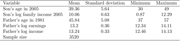
Table 1: Descriptive statistics: Characteristics of sons in the main sample
[image:12.595.82.497.202.290.2]Variable Mean Standard deviation Minimum Maximum Son’s age in 2005 39.36 5.64 30 49 Son’s log family income 2005 10.06 0.63 0.87 12.29 Father’s age in 1981 45.84 5.08 37 57 Father’s log earnings 13.2 0.36 12.34 14.11 Father’s log income 13.24 0.33 12.46 14.13 Sample size 3520
Table 2: Descriptive statistics: Characteristics of daughters in the main sample
Variable Mean Standard deviation Minimum Maximum Daughter’s age in 2005 39.55 5.66 30 49 Daughter’s log family income 2005 10.02 0.66 4.09 12.05 Father’s age in 1981 45.89 4.97 37 57 Father’s log earnings 13.21 0.36 12.34 14.11 Father’s log income 13.24 0.34 12.46 14.13
Sample size 3995
4
Results
4.1
Intergenerational earnings mobility for sons
In order to compare our results with the empirical literature on intergenerational
mobility, we present in this subsection our estimation of intergenerational earnings
mobility for sons. We use a two-sample two-stage estimation, whose first step consists
of the estimation of the paternal earnings regression using the supplemental sample,
and the results of this regression are presented in Table 3. These coefficients are then
used to impute the paternal earnings in the main sample, since we have the same
characteristics in both samples (main and supplemental). Therefore, in the second
step, using the coefficients from the supplemental sample and the characteristics of
the main sample, we estimate earnings for each father in the main sample.
Table 4 reports the second step, that is, the coefficients of the intergenerational
regression between annual sons’ earnings and the fathers’ imputed earnings. In all
columns, the father’s predicted log earnings has a significant positive effect on child’s
earnings.
We estimate the elasticity for sons for different age ranges. The ranges considered
are 30 to 40, 40 to 50, 30 to 50 (the whole sample) and a narrower range around 40
(those who are between 35 to 45). All the coefficients obtained are around 0.40 for all
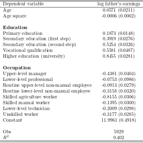
Table 3: First step: estimates of father’s earnings equation with the supplemental sample
Dependent variable log father’s earnings
Age 0.0571 (0.0211)
Age square -0.0006 (0.0002)
Education
Primary education 0.1873 (0.0148) Secondary education (first step) 0.3919 (0.0276) Secondary education (second step) 0.5254 (0.0326) Vocational qualification 0.5581 (0.0487) Higher education (university) 0.8455 (0.0281)
Occupation
Upper-level manager -0.4381 (0.0404) Lower-level professional -0.0753 (0.0986) Routine upper-level non-manual employee -0.0913 (0.0279) Routine lower-level non-manual employee -0.3158 (0.0320) Skilled agriculture worker -0.8155 (0.0306) Skilled manual worker -0.1395 (0.0300) Lower-level technician -0.2009 (0.0298) Unskilled worker -0.3177 (0.0285)
Constant 11.9961 (0.4918)
Obs 5929
R2
0.402
Note: Standard errors in parentheses. InEducation: none (reference) and inOccupation: Upper-level professionals (reference).
Table 4: Second Step: Intergenerational regression in annual earnings in the main sample for sons
Sons 30–40 Sons 40–50 Sons 30–50 Sons 35–45
Father’s earnings 0.38(0.042) 0.43(0.042) 0.40(0.029) 0.41(0.041) Age 0.14 (0.004) 0.02 (0.004) 0.02 (0.002) 0.02 (0.004) Constant 4.26 (0.597) 3.32 (0.603) 3.89 (0.413) 3.21 (0.585)
Obs. 1334 1322 2656 1501
R2
0.061 0.08 0.08 0.08
[image:13.595.124.476.581.681.2]we do not have enough information to know if it is due to a change in the trend such
that we will have more mobility or if it is only a matter of age in the sense that when
these young sons grow older they would become more correlated with their parents.
Once we have estimated our beta for sons is not immediate if the figure we get
means high or low mobility. We can use the figures reported in other studies to
compare. However, the comparability of studies is problematic and very difficult since
the estimates are sensitive to different factors such as the income measure used, the
adequacy of the database, the different criteria for sample selection and the different
estimation methods followed. Therefore, so as to compare our results with those of
other studies, we must be careful and choose the studies that are most similar to ours
in terms of choice of the sample, using two-sample approach.9
Fortunately, at present there are some studies that appear very close to our analysis
because they use similar methodologies and sample selection rules, allowing us to make
an international comparison. One of these papers is Bj¨orklund and J¨antti (1997) for
Sweden and the US. They find an elasticity of 0.52 for the United State and 0.28
for Sweden. Nicoletti and Ermisch (2007) apply the same methodology for Britain
and they obtain elasticities that ranges from 0.20 to 0.25 for sons. In the same way,
Lefranc and Trannoy (2005) for France, find an elasticity of 0.40 for sons. Furthermore,
Mocetti (2007) show Italy as a very immobile society. In particular, he finds elasticities
around 0.50.
As Lefranc and Trannoy (2005) point out, one possible explanation for why Europe
shows more intergenerational mobility than the United States is the way in which
higher education is financed. In Spain, France, and Sweden the access to higher
education is free, while in the United States payment of tuition may be a problem for
poor households, even if generous grants are available for bright students.
Evidence available for other countries and surveyed by Solon (2002) suggest a
rather high degree of intergenerational mobility in Finland ( ¨Osterbacka (2001)) and
Canada (Corak and Heisz (1999)), where the elasticity is around 0.2 or lower. There
9
is some empirical evidence for Germany (see Couch and Dunn (1997)) that expresses
a similar correlation to the United States.
Overall, we find an intergenerational correlation for Spain that ranks between a
group of more mobile societies, including the Nordic countries, Canada, and Britain
and a group of less mobile countries, which include the United States and Italy. We
find an elasticity that is similar to France for sons.
Tables A.2 and A.3 in Appendix A show the transition matrices for earnings and
education between fathers and sons. These tables give us an intuitive vision of the
persistence of earnings or education. Both tables show a strong degree of persistence.
If we consider the persistence of education as one of the mechanisms that enhances the
persistence of earnings, the design of education policies should take this into account
to increase mobility.
4.2
Intergenerational earnings and income mobility for
daugh-ters
As explained above, the empirical literature on intergenerational earnings mobility has
concentrated on the analysis of sons to avoid the employment selection problem. The
increase in female labour force participation in Spain began at the end of the 70s, but
this participation is still presently lower than that of men. It is intuitive that
full-time women workers are probably more common in some types of household (highly
educated households or very poor households).
However, in this subsection we want to give some insight into the
intergenera-tional earnings mobility for daughters. We deal with this selection problem following
Chadwick and Solon (2002) and using family incomes instead of daughter’s individual
earnings.10
In Table 5 we reproduce the Chadwick and Solon (2002) approach and we estimate
the elasticity between daughters (using different dependent variables) and fathers
earn-ings. In order to compare these results, we also do the same exercise for sons in Table
6.
In the first row of Table 5 and Table 6, we consider the log of family income as
10
Table 5: Intergenerational elasticity for daughters respect to their father’s earnings
Dependent variable Full daughters sample Married daughters Log family income 0.386 0.384
(0.028) (0.033)
Log couple’s earnings 0.497
(0.044)
Sample size 3995 1904
Note:Standard errors are corrected using Murphy and Topel (1985) and Inoue and Solon (2010) procedure.
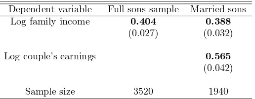
Table 6: Intergenerational elasticity for sons respect to their father’s earnings
Dependent variable Full sons sample Married sons Log family income 0.404 0.388
(0.027) (0.032)
Log couple’s earnings 0.565
(0.042)
Sample size 3520 1940
Note:Standard errors are corrected using Murphy and Topel (1985) and Inoue and Solon (2010) procedure.
a dependent variable. In the second row, we restrict the sample to those who are
married and we consider the log of the couple’s combined earnings.
Concretely, we present the results of the estimation of equation 5 by the TSTSLS
estimator with different dependent variables and samples. We begin (in the first row,
first column of Table 5) with the estimation of the elasticity of daughter’s family
income with respect to her father’s earnings for our full sample of 3995 daughters
and we obtain an elasticity of 0.38. As we can see in Table 6, for the full sample of
3520 sons, we find an elasticity of 0.40. Therefore, the elasticities between daughter’s
and father’s earnings are very little smaller than the sons’ elasticity, however not
statistically different.11
When we do the same, but considering only daughters who are married (first row,
second column) with respect to paternal earnings in Table 5, we obtain a very similar
elasticity of 0.384.12 For sons we estimate an elasticity of 0.388. Again, the results
11
The t-ratio for the contrasts between these two coefficient is 0.46, so the contrast is not statistically significant at conventional significance levels.
12
[image:16.595.171.429.263.364.2]obtained are very similar by genders.
For married daughters and sons we also analyse the paper of couple’s earnings.
Therefore, in the second row of each table we estimate the elasticity between couple
earnings (the log of the sum of the daughter’s earnings and her husband’s earnings) and
paternal earnings. In this case the elasticities increase to 0.50 for married daughters
and 0.57 married sons. The figure 0.57 may seem relatively high compared to 0.50,
and higher mobility for daughters is also found in Chadwick and Solon (2002) and
Ermisch, Francesconi, and Siedler (2006), but the t-ratio of 1.12 again did not allow
us to reject the null hypothesis of equal coefficients.
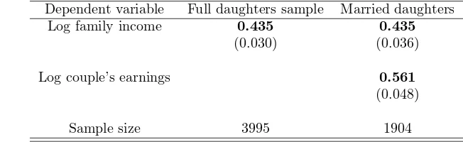
In Table A.4 and Table A.5 in Appendix A, we present the same exercise using
paternal income as an explanatory variable. Again we obtain results in the same
direction.
5
Final remarks
In this paper, we contribute to the empirical literature that calculate the
intergener-ational mobility for different countries estimating the earnings and income elasticity
for Spain. Using the two-sample two-stage least squares estimator, we find sons’
elas-ticities around 0.40. Using Chadwick and Solon (2002) approach and comparing the
estimates for sons and daughters, our results suggest that elasticities for both genders
are nearly the same.
Where does Spain fit into the larger picture of intergenerational mobility? In some
ways, it’s in the middle. It is similar to France, lower than the Nordic countries and
Britain, and higher than the United States. Compared to other developed countries,
Spain is relatively immobile, but it is more mobile than Italy, the only other southern
Appendix A
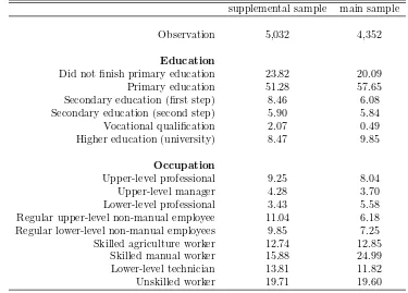
Table A.1: Distribution of father’s education and occupation as well as coincidences between supplemental and main sample
supplemental sample main sample
Observation 5,032 4,352
Education
Did not finish primary education 23.82 20.09 Primary education 51.28 57.65 Secondary education (first step) 8.46 6.08 Secondary education (second step) 5.90 5.84 Vocational qualification 2.07 0.49 Higher education (university) 8.47 9.85
Occupation
Upper-level professional 9.25 8.04 Upper-level manager 4.28 3.70 Lower-level professional 3.43 5.58 Regular upper-level non-manual employee 11.04 6.18 Regular lower-level non-manual employees 9.85 7.25 Skilled agriculture worker 12.74 12.85
Skilled manual worker 15.88 24.99 Lower-level technician 13.81 11.82 Unskilled worker 19.71 19.60
Table A.2: Transition matrices of earnings between fathers and children
Father’s quantile
1 2 3 4 5
Quantile of the son or daughter
[image:19.595.125.474.254.338.2]1 30,08% 23,93% 16,98% 16,20% 13,23% 2 24,40% 22,34% 19,17% 18,29% 16,20% 3 19,12% 23,54% 20,26% 21,67% 15,66% 4 15,74% 15,69% 22,64% 23,26% 22,41% 5 10,66% 14,50% 20,95% 20,58% 32,49%
Table A.3: Transition matrices of education between fathers and children
Father’s education
0 1 2 3 4 5
Child’s education
1 34,07% 13,89% 4,85% 3,04% 0,00% 0,60% 2 34,77% 23,72% 18,12% 7,43% 8,00% 3,99% 3 17,98% 25,22% 34,30% 31,42% 36,00% 16,37% 4 1,90% 2,18% 1,94% 1,01% 12,00% 1,00% 5 11,29% 34,98% 40,78% 57,09% 44,00% 78,04%
Table A.4: Intergenerational elasticity for daughters with respect to their father’s income
Dependent variable Full daughters sample Married daughters Log family income 0.435 0.435
(0.030) (0.036)
Log couple’s earnings 0.561
(0.048)
[image:19.595.124.450.415.515.2]Table A.5: Estimated intergenerational elasticity for sons and daughters with respect to their father’s income
Dependent variable Full sons sample Married sons Log family income 0.461 0.455
(0.030) (0.034)
Log couple’s earnings 0.653
(0.046)
Sample size 3520 1940
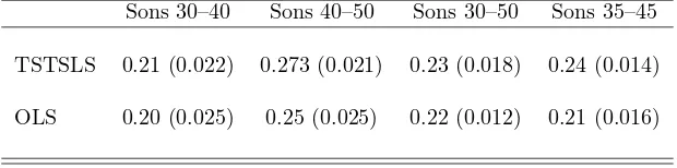
Appendix B
As we explain in Section 2.2, the TSTSLS estimation could produce an
overesti-mation of β when the variables used to impute father earnings are endogenous and
do not perfectly explain father earnings. In order to measure the potential bias of
the TSTSLS, we can use the restricted sample of father-son pairs who co-reside and
compare the estimates using OLS and TSTSLS.
The estimation results are reported in Table B.1
Table B.1: Intergenerational earnings elasticity for father-son pairs who co-reside
Sons 30–40 Sons 40–50 Sons 30–50 Sons 35–45
TSTSLS 0.21 (0.022) 0.273 (0.021) 0.23 (0.018) 0.24 (0.014)
OLS 0.20 (0.025) 0.25 (0.025) 0.22 (0.012) 0.21 (0.016)
Note: The dependant variable is the log of annual labor earnings. Father’s earnings refers to the log of father’s annual labor earnings. Standard errors are corrected using Murphy and Topel (1985) and Inoue and Solon (2010) procedure.
We do not find evidence of a large amount of upward bias. This results are in line
[image:20.595.143.453.437.514.2]References
Aaronson, D., and B. Mazumder (2008): “Intergenerational economic mobility in the United States, 1940 to 2000,” Journal of Human Resources, 43(1).
Angrist, J. D., and A. B. Krueger (1992): “The effect of age at school entry on educational attainment: an application of instrumental variables with moments from two samples,” Journal of the American Statistical Association, 87, 328–336.
Arellano, M., and C. Meghir (1992): “Female labour supply and on-the-job search: an empirical model estimated using complementary data set,” The Review of Economic Studies, 59, 537–559.
Behrman, J. R., and P. Taubman (1990): “The intergenerational correlation between children’s adult earnings and their parents’ income: results from the Michigan Panel Survey of Income Dynamic,” Review of Income and Wealth, 36(2), 115–127.
Bj¨orklund, A., and M. J¨antti (1997): “Intergenerational income mobility in Sweden compared to the United State,”American Economic Review, 87, 1009–1018.
(2000): “Intergenerational mobility of socioeconomic status in comparative per-spective,”Nordic Journal of Political Economy, 26(1), 3–32.
Bowles, S., and H. Gintis (2002): “The inheritance of inequality,”Journal of Economic Perspectives, 16, 3–30.
Caraba˜na, J. (1999): Dos estudios sobre movilidad intergeneracional. Fundaci´on Argendaria-Visor (ed.).
Chadwick, L., and G. Solon (2002): “Intergenerational income mobility among daugh-ters,” American Economic Review, 92(1), 335–344.
Corak, M., and A. Heisz(1999): “The intergenerational earnings and income mobility of canadian men: evidence from longitudinal income tax data,”Journal of Human Resources, 34(3), 504–533.
Couch, K., and T. Dunn (1997): “Intergenerational correlations in labor market status: a comparison of the United State and Germany,” Journal of Human Resources, 32(1), 210–232.
Erikson, R., and J. H. Goldthorpe(2002): “Intergenerational inequality: a sociological perspective,”Journal of Economic Perspective, 16, 31–44.
Ermisch, J., M. Francesconi, and T. Siedler (2006): “Intergenerational economic mobility and assortative mating,” Economic Journal, 116, 659–679.
Fortin, N., and S. Lefebvre (1998): “Intergenerational income mobility in Canada,” in
Labour Market, Social Institution and the Future of Canada’s Children, ed. by M. Corak. Statistics of Canada, Ottawa.
Grawe, N.(2004): “Intergenerational mobility for whom? The experience of high- and low-earnings sons in intergenerational perspective,” inGenerational Income Mobility in North America and Europe, ed. by M. Corak. Cambridge University Press, Cambridge.
Haider, S., and G. Solon(2006): “Life-cycle variation in the association between current and lifetime earnings,” American Economic Review, 96(4), 1308–1320.
Inoue, A., and G. Solon (2010): “Two-sample instrumental variables estimators,” The Review of Economics and Statistics, 92(3), 557–561.
Lefranc, A., and A. Trannoy (2005): “Intergenerational earnings mobility in France: Is France more mobile than the U.S.?,”Annales d’Economie et de Statistique, (78), 03.
Mocetti, S. (2007): “Intergenerational Earnings Mobility in Italy,” The B.E. Journal of Economic Analysis & Policy, 7: Iss. 2 (Contributions), Article 5.
Murphy, K. M., and R. H. Topel(1985): “Estimation and inference in two-step econo-metric models,” Journal of Business & Economic Statistics, 3(4), 370–79.
Nicoletti, C., and J. Ermisch (2007): “Intergenerational earnings mobility: changes across cohorts in Britain,”The B.E. Journal of Economic Analysis and Policy. Contribu-tions, 7: Iss. 2 (Contributions), Article 9.
Nicoletti, C., and M. Francesconi (2006): “Intergenerational mobility and sample selection in short panels,”Journal of Applied Econometrics, 21(8), 1265–1293.
¨
Osterbacka, E.(2001): “Family background and economic status in Finland,” Scandina-vian Journal of Economics, 103(3), 467–484.
Piraino, P.(2007): “Comparable Estimates of Intergenerational Income Mobility in Italy,”
The B.E. Journal of Economic Analysis & Policy), 7: Iss. 2 (Contributions), Article 1.
Ridder, G., and R. Moffit (2006): “The econometrics of data combination,” in Hand-book of Econometrics, ed. by Heckman, and Learner, 6. Elsevier Science, North Holland, Amsterdam.
Sanchez-Hugalde, A. (2004): “Movilidad intergeneracional de ingresos y educativa en Espa˜na (1980-90),” Discussion paper.
Solon, G. (1992): “Intergenerational income mobility in the United States,” American Economic Review, 82(3), 393–408.
(1999): “Intergenerational mobility in the labour market,” in Handbook of Labor Economics, ed. by O. Ashenfelder, and D. Card, vol. 3, chap. 29, pp. 1761–1800. Amster-dam: Elsevier.
(2002): “Cross-country differences in intergenerational earnings mobility,”Journal of Economic Perspective, 16(3), 59–66.