Voting with Your Feet: Political Competition and Internal Migration in the United States

Munich Personal RePEc Archive

Voting with Your Feet: Political

Competition and Internal Migration in

the United States

Liu, Wai-Man and Ngo, Phong

Australian National University

16 October 2012

Online at

https://mpra.ub.uni-muenchen.de/43601/

Voting with Your Feet: Political Competition and

Internal Migration in the United States

Wai-Man Liu

Australian National University

Phong Ngo

Australian National University

Abstract

Do people "vote with their feet" due to a lack of political competition? We

formal-ize the theory of political competition and migration to show that increasing political

competition lowers political rent leading to net in-migration. Our empirical

appli-cation using US data supports this prediction. We …nd that an increase in political

competition - in the order of magnitude observed in US Southern states during the

post-war period - leads to an increase in net migration of approximately 36 individuals

per 1000 population. In comparison, birth rates over the last century ranged between

70 and 150 births per 1000 population.

JEL Classi…cation: D72, J61, H70, N92

Key Words: political competition, internal migration, welfare, Voting Rights Act.

We are grateful to Professor James Snyder for proving us with the U.S. state election data. We thank Tim Hatton, Aaron Bruhn, Umit Gurun, Michelle Lowry and seminar participants from the Australian National University and the Australian Department of Education, Employment and Workplace Relations for helpful comments and discussions.

1

Introduction

Economic orthodoxy suggests that a lack of competition allows …rms to restrict output

and raise prices ine¢ciently. Competition, on the other hand, is welfare enhancing since

it allows consumers to switch producers if their current supplier increases prices. Whether

a lack of competition between political parties has similar welfare destroying e¤ects leading

voters to "vote with their feet" by moving to a more politically competitive domain is far less

discussed. Moreover, the empirical literature on the determinants of migration is virtually

silent on whether political competition matters for migratory choices.

Accordingly, we develop and test a general equilibrium model with endogenous structure

of division of labor to formalize the theory of political competition and migration. The

technical substance of our model is inspired by a model of implicit corruption developed

in Yao (2002a). In an economy, each individual is a consumer-producer who can choose

her number of goods purchased and her number of goods self-provided, which determine her

level of specialization. Each consumer-producer prefers diverse consumption and specialized

production due to economies of specialization in producing each good. We assume that

there is an occupation providing public goods (…nanced by tax), such as administration of

infrastructure, judicial services, law enforcement, and transaction services. Individuals must

consume public goods when they trade goods in the market, and these public goods a¤ect

the transaction cost associated with trades. Hence, there is a trade-o¤ between economies

of division of labor and transaction costs. Because of this trade-o¤, as the transaction cost

for a unit of traded good decreases, the equilibrium level of division of labour and extent of

the market increase.

First consider a setting where there is free entry into every occupation including the

public sector (politically competitive). Free entry into each occupation, and ‡exible prices

and tax, generate an equilibrium that not only sorts out the e¢cient resource allocation, but

also determines an e¢cient level of division of labor, by trading o¤ economies of division of

that for public goods. The equilibrium level of division of labor and resource allocation

under this setting is Pareto e¢cient.

We then consider a setting where there is limited competition in the political arena. In

this setting, tax is not determined by free entry into the public sector. Instead, there is a

group of individuals (we call it the elite group) who produce the public goods and manipulate

the tax they charged by blocking entry into the public sector and indirectly manipulate the

output of public goods relative to outputs in other sectors. The ine¢cient supply of public

goods creates rents that make per capita real income of the elite group much higher than

that of commoners. This distorted terms of trade restricts the extent of the market, and

lowers the equilibrium level of division of labor. Because of economies of division of labor,

the equilibrium level of aggregate productivity in this setting is not Pareto optimal. Within

the state, the degree of rent extraction depends on the commoners’ level of intolerance for

such behaviour by the politically elite - one can think of intolerance being determined by

factors such as education, political ideology, social norms, cultural/moral codes, and religion.

Allowing for multiple states with free migration, we consider the impact of an increase

in one state’s level of political competitiveness on migration between states. We show that

increasing political competition lowers political rent leading to net in-migration to the state,

which in turn promotes economic development through a higher level of division of labor.

That is, political competition is positively associated with net migration.

The application of our model tests this key prediction. We exploit the signi…cant

cross-state and within-cross-state variation in political competition to explain internal (cross-state-to-cross-state)

migration in the United States (US) using two sources of migration data: (1) Census data,

1940-2010; and (2) the Internal Revenue Service (IRS), 1988-2010. A consistent picture

emerges: political competition is positively related to net migration - that is, individuals tend

to migrate to more politically competitive states and away from politically uncompetitive

states. This result is robust to multiple proxies for net migration, model speci…cations and

and with controls for economic and demographic factors. We estimate this model, with

and without lagged net migration terms using System-GMM (Arellano and Bond, 1991;

Arellano and Bover, 1995; Blundell and Bond, 1998) and least squares respectively. Second,

our results are robust when we instrument for political competition to alleviate concerns

about reverse causality - indeed, our general equilibrium model predicts a feedback e¤ect

from migration to political competition. Third, we perform a similar analysis using annual

internal migration data from the IRS and …nd similar results.

Our …ndings are not only statistically signi…cant but also economically meaningful.

Us-ing …ve-year migration rates from the Census data we …nd that an increase in political

competition of 0.3 (common among Southern states of the US for the post war period) leads

to an increase in net migration of approximately 36 individuals per 1000 population. To

put this in context, …ve-year birth rates over the last century ranged from a maximum of

150 per 1000 population to 70 per 1000 population.

Our work is related to several streams of literature. First, our model reinforces the ideas

of early scholars on the relation between political competition and development - broadly

de…ned (see the discussion in Liu and Yang (2007) and the references therein). For example,

Baechler (1976, pg. 80) famously argued:

“[f]undamental springs of capitalist expansion are, on the one hand, the

coexis-tence of several political units within the same cultural whole and on the other,

political pluralism which frees the economy.”

More recently, Polo (1998) and Svensson (1998) develop models showing that a lack of

political competition can lead to excessive rent-seeking behaviour or the ine¢cient provision

of public goods. The latest contribution to this area is a paper by Besley et al. (2010),

who develop a model showing that political competition forces politicians to pursue growth

promoting policies which in turn leads to better economic outcomes. They test their model

using US data and …nd compelling evidence in favor of their conjecture. Our empirical

Second, while our model is closely related to Li and Smyth’s (2004) model that shows

how competitionbetween the two states generated by free migration results in more e¤ective

third party protection for property rights, which in turn promotes division of labour and

specialization, our model is di¤erent from their’s in two ways. First, our emphasis is

on the migratory response to the level of political competition within the state. Second,

their model considers two consumer goods, which yield limited implications on the e¤ect

of political competition on the extent of the market. Our model considers m goods and furthermore, it simultaneously endogenizes the level of division of labor, the extent of the

market, the degree of inequality of income distribution and economic performance. Our

paper is also related to Acemoglu and Robinson’s (2000) theoretical work on explaining why

the west extended the franchise in the nineteenth century. They argue that the decision to

extend voting rights is endogenously determined because of the fear of social upheaval. Our

application uses the 1965 Voting Rights Act to instrument for political competition (more

on this below). Unlike Acemoglu and Robinson’s (2000) argument, this law change was

exogenous to state-level politics, since it represented a federal intervention into Southern

state politics rather than a decision by Southern states to extend voting rights.

Third, our model reinforces Charles M. Tiebout’s (1956) pioneering work on competition

for public goods provision. Under a set of rather strict assumptions, Tiebout establishes a

simple equilibrium model of how consumer-voter’s voluntary mobility decision determines

the size of local governments (or local communities). Unlike Tiebout’s theory, which takes

as given the bundle of taxes and public goods in each location, and then considers

competi-tion between locations, our model studies how political competition within a given location

endogenously determines the level of taxation and publics goods, before considering the

mi-gratory responses of individuals in response to di¤erences in political competition (and hence

bundle of taxes and public goods) across locations.

Finally, our work contributes to empirical literature on the determinants of internal

migrate. This literature is vast so we do not attempt to provide a complete review (see

Greenwood 1975; Greenwood 1985; and Greenwood 1997 for extensive reviews). Research

on the determinants of migration is typically formulated in the context of individual utility

maximization, with early contributions to the literature focusing on economic di¤erences

between origin and destination as key drivers. Later research has emphasized the

impor-tance of non-economic factors such as disimpor-tance, personal characteristics and life cycle e¤ects,

weather and the environment (Banzhaf and Walsh, 2008), the business cycle (Saks and

Wozniak, 2011), and taxes and the availability of public goods (Banzhaf and Walsh, 2008).

None however, explicitly look at the impact of di¤erences in political competition between

locations on migratory choices.

The remainder of the paper is organized as follows. Section 2 presents the model.

Sec-tions 3 provides some historical background and discusses measurement of our key variables,

political competition and internal migration in the US. Section 4 discuss the empirical

methodology and the results. Section 5 concludes the paper.

2

Model

Consider a state (k) which has a continuum of consumer-producers of mass Mk, withmk

consumer goods. For reasons of notational convenience, we drop k in this section. The state subscript will be used later, when we derive the endogenous population size caused by

migration. We assume the absence of a dichotomy between consumers and producers to allow

individuals to choose their levels of self-su¢ciency, or its reciprocal: levels of specialization.

We can then formalize Allyn Young’s (1928) idea that individual choices of their level of

specialization generates network e¤ects which imply that each person’s specialization decision

depends on the number of participants in the network of division of labor (the extent of

the market), while this number is in turn determined by the specialization decisions of all

on the extent of the market, but the extent of the market is also determined by the level

of division of labor). Each consumer-producer has the following ex ante identical utility

function

(1) u=

m

Y

i=1

(yi+Kiydi):

where yi is the amount of good i self-provided, yd

i is the amount of good i purchased from

the market. Ki is a fraction of a unit of good ipurchased that disappears in transit because of transaction cost. Hence,K can be interpreted as a trading e¢ciency coe¢cient of a unit of goods purchased.1 _{We assume that Ki is increasing in the amount of public goods, gi,} provided by the state, and the public good is consumed exclusively within each respective

state. For the sake of simplicity, let

(2) Ki =gi:

We consider the sector providing the public goods as political, administrative, judicial, and

law enforcement services that a¤ect trading e¢ciency.2 _{The production of this service}

in-volves primarily …xed costs but negligible variable costs, which implies signi…cant increasing

returns. We assume the state is a monopoly supplier of the transaction service and prices

the service indirectly via bundling (implicitly) with other services and taxation.

Suppose, there is free entry into any sector including the public sector. yi+Kiyd

i is then

the amount of good i that is received for consumption. Each individual has the following system of production functions for good i and transaction services k:

(3a) yi+ys

i = maxf0; li ag, for a2(0;1);

1_{The speci…cation of such "iceberg" transaction costs is common practice in equilibrium models with a}

trade-o¤ between increasing returns and transaction costs (see Krugman,1995). This speci…cation avoids the notoriously formidable index sets of destinations/origins of trade ‡ows.

2_{In this paper, we do not speci…cally model the public good nature of the transaction service. We leave}

(3b) gi = maxf0; lgi bg, forb 2(0;1):

where a and b are the …xed learning costs of producing a good and transaction service, respectively. li and lgi are the amount of labour allocated to the production of good i

and public goods, respectively. ys

i is the amount of good i supplied to the market. Each

individual is endowed with one unit of working time, and the endowment constraint is:

(4) P_ili +P_ilgi = 1, for li; lgi 2[0;1];

The above system of production functions displays economies of specialization; that is,

each person’s labor productivity increases as her scope of production activities narrows

down since her total …xed learning cost decreases and thereby her production time increases

as she becomes more specialized.3 _{Here, the endowment of labor is speci…ed for each}

person since the learning by doing process, which generates economies of specialization,

is individual speci…c and cannot be transferred between individuals. This implies that

economies of specialization are localized increasing returns which are compatible with a

competitive market. The budget constraint is given by:

(5) Pn_i piyd

i =

Pn i piy

s

i(1 t),

where pi is the price of good i. The government charges proportional tax on sales income (sales tax). Let t be the tax rate: t 2(0;1). Because the public good is non-rivalrous and non-excludable, we assume the cost of enforcing the property rights of good g is too high. Hence, the government cannot charge a tax per usage of the good.

Each consumer-producer maximizes her utility with respect to yi, yd

i, yis, yj, gi, li, lj, lgi 0, subject to the production functions, the endowment constraint, and the budget

constraint. Since all decision variables can take on zero value, each individual’s decision

problem is a nonlinear programming problem. There are 4m independent decision variables

yi, yd

i, yis, gi (li, lg are not independent of the other decision variables). Each of them can

be either positive or zero. Hence, there are24m _{possible interior and corner solutions of the}

nonlinear programming problem. Let us assume the public good is homogeneous across good

i. Hence we can use lg instead of lgi. We use the theorem of optimal con…guration (Wen,

1998 and Yao, 2002b) to rule out many combinations of the interior and corner solutions.

According to this theorem, an optimal decision does not involve selling and buying the same

goods, does not involve self-providing and buying the same good, and sells at most one good

although many goods can be produced and self-provided. This theorem, together with the

budget constraint and a positive utility requirement, imply that we can divide the population

into many occupations. Each occupation is characterized by the good sold by a specialist

choosing this occupation. It implies that for a person selling good i, her occupation is characterized by

yi; yj; yd r; y

s

i; li; lj; gr >0; yr; yid; y

s

r; lr; lg; y d j; y

s

j = 0 for8r 2 R and 8j 2 J,

(6a)

whereRis the set ofn 1goods that are purchased from the market andJ is the set of non-traded goods. The individual specialist produces and supplies good i (yi; ys

i >0), demands

good r (yd

r), for r 6= i, and produces non-trade good j (yj). She uses public goods gr for

each purchase of good r. The decision con…guration of individuals providing public goods, who might be government o¢cials, politicians, public administrators, middlemen, judges,

lawyers, policemen, and infrastructure builders, di¤ers from that of sellers of goods. She

specializes in producing and selling transaction services; she has no demand for transaction

de…ned by the following conditions:

yj; yd

r; lg; lj >0; yr; ys

r; lr; y d j; y

s

j = 0 for 8r2 R

0

and 8j 2 J, (6b)

whereR0

is the set ofn goods that are purchased from the market by a specialist provider of public goods. Note that a specialist provider of public goods does not sell any good. Hence,

she buys allntraded goods. Without loss of generality, we assume each person trades goods

1;2; :::; n and self-provides goods n+ 1; n+ 2; :::; m.

Using the condition (6a) and invoking the symmetry of the model, the decision problem

for commoners (or a consumer-producer selling good i) is:

(7) maxuy =yi(gryrd)

n 1_ym n j ;

subject to the production function for traded goodiand non-traded goodj, the endowment constraint and the budget constraint:

yi+ysi = maxf0; li ag;

yj = maxf0; lj ag;

li+ (m n)lj = 1;

(n 1)pryd r =p1y

s

1(1 t):

pi and pr are the price of goodi and good r, respectively,8r 2 R. Under this speci…cation, the consumer-producer self-provides and sells one …nal good; buysn 1…nal goods andn 1

transaction services forn 1goods purchased from the market. t is the proportional tax on sales income.

occupation until utility is equalized across occupation. Let n indirect utility functions, which involve relative prices of n traded goods to be equalized. We can obtain symmetric equations. These equations hold simultaneously only if prices of all traded goods are the

same. Hence, we have pi = pr for anyi and r. Using this symmetry, we can simplify the decision problem of a representative consumer-producer selling a good (for instance, good

1). The unconstrained optimization problem for the consumer-producer is:

(8) max

l1;y1s

uy = (l1 a ys1)gn 1

pr p1

ys

1

(n 1)(1 t) n 1

1 l1

m n a

m n

.

The …rst order conditions for the optimization problem yield the demand functions for good

r,yd

r, the supply function of good 1,ys1, and the optimal amount of labor allocated to produce

good 1,l1. Inserting them back into the utility function, the utility of the consumer-producer

as a function of a, m, n, g and t can be expressed as follow:

(9) uy = 1 a(m n+ 1)

m

m

gn 1_{(1 t)}n 1_:

The above utility function shows that the per capita consumption of each good or service is

[1 a(m n+ 1)]=m, where1 a(m n+ 1) is the time allocated to produce the good sold and m n non-traded goods after the total …xed learning cost is deducted. As n increases, the amount of time available for the production increases as the total learning cost incurred

for non-traded goods production, a(m n) reduces. The denominator shows the person’s total number of types of goods and services, which includes: (i) m n non-traded goods; (ii)n 1traded goods bought in the market; and (iii) one self-provided good, which is sold as well. Additionally, the person consumesn 1public goodsg. Since the marginal labor productivity of each good is 1, the per capita consumption can be considered also as the per

capita output of each good or service. Let us now consider the decision problem for a person

the model, her constrained optimization problem is:

(10) maxug = (gryd

r)nyjm n,

subject to the production functions for public goodg and non-traded goodj, the endowment constraint and the budget constraint:

g = maxf0; lg bg;

yj = maxf0; lj ag;

lg+ (m n)lj = 1;

npiyd

i =npiy s it:

The public servant buys n traded goods. Each traded good requires public goods g gr

to facilitate the transaction. Additionally, she produces m n non-traded goods. Her unconstrained optimization problem is:

(11) max

lg

ug = (lg b)n(ysit)

n 1 lg

m n a

m n :

Due to symmetry, we omit subscript r from g when no confusion is caused. The …rst order conditions for the optimization problem (11) yield the optimum level of specialization

in producing the public goods lg. Cross substituting these solutions we can express the utility of the public servant as a function of relative prices, a, b,m, and n.

(12) ug = 1 b a(m n)

m

m

[1 a(m n+ 1)] m

n

(n 1)nnn_tn_:

function of a, m, n, and t,

(13) uy = 1 a(m n+ 1)

m

m

1 b a(m n) m

n 1

nn 1_{(1 t)}n 1_:

Suppose that there is free entry into each occupation including the public sector

(politi-cally competitive). Free entry implies that the utility of a person selling a consumer good

and a person producing the public goods must be equalized. That is:

(14) uy =ug.

Free entry also implies that the price and the tax rate are determined when all

consumers-producers behave competitively. If the public sector yields a higher utility than other sectors

because of a higher tax, competitive entry to public sector will drive up the supply of the

public goods and drive down the tax rate until utility between the public sector and other

sectors are equalized. The utility equalization condition (14) yields the optimal tax rate t , which is obtained by solving (15).

(15) t nn1 +At A= 0;

whereA m

1

n 1

nn11_{(n 1)}nn1 [1 a(m n+ 1)]

m n n 1

h

1 1 b a(m n)

im n+1

n 1

. Substitutingt into (12) yields the equilibrium utility which will give utility as a function ofn:

(16) u(t (n); n):

The e¢ciency theorem (see Yang and Liu (2009, pg. 70)) shows that the general

equilib-rium in such a model with an endogenous structure of division of labor is the Pareto corner

is determined by a value of n that maximizesu(t (n); n):

(17) dug(t (n ); n )=dn = 0;

and the solution yields the equilibrium number of traded goodsn as a function of a,b and

m. Inserting n (a; b; m) into (16) yields equilibrium per capita real income when the state is competitive. The level of division of labor and the extent of the market are characterized

byn (a; b; m). It represents the number of di¤erent traded goods, which relates to diversity of occupations. It positively relates to each person’s level of specialization.4

A general equilibrium is de…ned by relative prices and numbers of individuals choosing

various occupations and associated quantities of goods produced, traded, and consumed, that

satisfy the following conditions: (i) Each individual chooses her labour allocation among all

production activities of goods and services and her trade plan, which generate her

consump-tion bundle, to maximize her utility for given prices of traded goods and given numbers of

individuals choosing various occupation con…gurations. (ii) The prices of traded goods and

numbers of individuals choosing various occupations clear all markets.

LetMk;i be the number (measure) of individuals selling goodiin state k. Recall thatgi

is non-rivalrous and non-excludable and thus there is no market for it. The market clearing

conditions for good i is given by:

(18) Mk;iys

i =

P

r2RMk;ry

d

i(r) +Mk;gy d

i(g), 8i= 1;2; :::; n;

where i is an element of the index set of n traded goods, yd

i(r) and ydi(g) are the demand 4_{As shown in Yang (1996, 2001, ch. 11), each individual’s level of specialization, the extent of the market}

function for good i by a person selling good r, and public goods g, respectively. Due to symmetry, P_r2RMk;ry

d

i(r) = (n 1)Mk;ryid(r). One of n + 1 equations in (18) is

not independent of other equations due to Walras’ law. The n independent equations, together with the population size identityP_sMk;s =Mk, wheres = 1;2; :::; n; g, yield the n

equilibrium numbers of specialists sellingn traded goods and the number of public servants providing public goods. Let Mk;y be the number of specialists selling a traded good. The symmetry of the market clearing conditions across goods generates the number of public

servant relative to the number of specialists selling a traded good (or the relative size of the

government):

(19) Mk;g

Mk;y = 1;

as yd

i(g) =yist and yid(r) = yis(1 t)=(n 1).

2.1

Equilibrium when the state is not politically competitive

Suppose the ruling elites of the state have the ability to team up and e¤ectively block

the entry into the public sector. They do so by manipulating the number of ruling elite

members relative to specialists in other occupations (commoners). A historical example,

which we discuss in more detail below, is how the Democratic party in the US Southern

states e¤ectively eliminated political competition between 1890 and 1960 by introducing

various voting restrictions that impacted on the poor and black population who made up

the support base for the Republican party.

To maximize utility of each member of the elite group, to the extent that commoners

do not choose to migrate to another location, the ruling elites extract political rent from

commoners by charging a high tax (or providing a low quality public goods).

Since there is no free entry into the elite group, the state is, by de…nition, not politically

utility function of the ruling elites is an increasing function of tax relative to the price of

goods bought, their utility increases and the commoner’s utility decreases as the relative size

of elite group to commoners decreases. De…ne as the intolerance level of commoners. If

commoners’ utility falls below , they will migrate away. Hence, the non-migration constraint

is:

(20) uy .

Exogenous factors such as education, political ideology/freedom, social norms, cultural/moral

codes, and religion of individuals in the society determine intolerance levels( ). Since

max-imization of the ruling elite’s utility is equivalent to the minmax-imization of a commoner’s, the

ruling elite group will manipulate relative size of public sector to other sectors until:

(21) uy = .

If is low, the level of political competitiveness within the state tends to be low because the

ruling elites can extract more rent from commoners, where the rent equals to the di¤erence

between ug and as:

(22) ug > uy = :

uy and ug are derived in the same way as outlined in previous section. The intolerance constraint (21), together with utility equalization conditions across all occupations of

com-moners, yields the optimal tax rate, t, which is a function of :

(23) t= 1 n11 (n):

where (n) mm

+n 1

n 1

n [1 a(m n+ 1)]

m

rate, the utility of the public servant is:

ug(t( ; n); n; ) = 1 b a(m n) m

m

[1 a(m n+ 1)] m

n

(n 1)nnn

h

1 n11 (n)

in :

(24)

The equilibrium level of division of labornis a function of , given by the …rst order condition:

(25) dug(n( ); )=dn= 0:

If education, political ideology/freedom, social norms, cultural moral codes, and religion

cause individuals to have a low level of intolerance, the level of political competitiveness

within the state is low and the ruling elites will use their monopoly power for rent seeking.

This rent seeking behavior by the elite group is called state opportunism, which is considered

by North and Weingast (1989) and Sachs, Woo, and Yang (2000) as a major obstacle of

economic development. Further, political competition promotes a higher level of division

of labor in the economy through a lower political rent. A higher level of division of labor,

represented by a larger number of traded goods, means higher aggregate productivity in our

model of endogenous structure of division of labor. We now establish the …rst proposition.

Proposition 1. Lower political competitiveness is associated with a higher tax rate, inferior

economic performance and a higher degree of inequality of income distribution (between the

ruling elite and commoners).

Proof See Appendix A.

This result reinforces earlier work by Polo (1998), Svensson (1998) and Besley et al.

(2011) who develop models showing that a lack of political competition can lead to

exces-sive rent-seeking behaviour, the ine¢cient provision of public goods and inferior economic

We now extend the model to consider a two-states case (k = 1;2). Let M be the mass of a continuum of consumer-producers, forM =M1+M2. There is no goods trade between

the states (and public goods produced within the state can only be consumed locally) but

individuals are free to migrate between states. The opportunity cost of immigration depends

on . The non-migration constraint (20) is rewritten as follows:

(26a) uy;1 maxf 1; uy;2g;

(26b) uy;2 maxf 2; uy;1g:

Consider an increase in the degree of political competitiveness of one state relative to

the other, holding all else constant. We model this through an increase in the level of

intolerance, k, in one state relative to the other. This exogenous increase in kis empirically

akin to the introduction of the 1965 Voting Rights Act which, for the …rst time, allowed full

political participation for the poor and black population in Southern US states (more on

this below). In contrast to Acemoglu and Robinson’s (2000) argument that the decision to

extend voting rights could be endogenous because of the fear of social unrest and revolution,

the introduction of 1965 Voting Rights Act is an exogenous event since it is a nationwide

prohibition of the denial or abridgment of the right to vote. It gave the Attorney General

the right to challenge any discriminatory voting practices in state or local election in the

court of law. From the non-migration constraints above, this raises uy;k since the political elite must allow entry into the public sector which leads to less rent extraction. We now

establish our second proposition.

Proposition 2(Voting with your feet).Ceteris paribus, an increase a state’s level of political

competitiveness, increases inward migration relative to the other state.

This proposition is the key prediction we focus on in our empirical testing: that political

competition is positively related to net migration.

In our general equilibrium model, an increasing population, in turn, promotes economic

development through a higher level of division of labor. Such an increase will foster market

integration, enhance production concentration, utilize endogenous comparative advantage

and increase occupation diversity in the economy.

Finally, we show that in equilibrium, an increase in the level of political competitiveness

in one state will increase the level of political competitiveness in competing state because of

the threat of out-migration.

Proposition 3. An increase in the level of political competitiveness in one state will increase

the level of political competitiveness in competing state because of the threat of outward

mi-gration. The ruling elites will lower the political rent extraction through a lower tax rate.

Consequently, income inequality will be lowered and economic performance will be improved.

Proof See Appendix A.

This result naturally follows due to our general equilibrium framework. Empirically,

testing this proposition is outside the scope of this paper, however, it does suggest an avenue

for future empirical work studying the consequences of migration. This literature is in

itself large and diverse, however, there is no systematic study on the impact of migration on

political outcomes.

3

Internal Migration & Political Competition

Internal migration has a long history of being a de…ning characteristic of the US economy.

Enhanced mobility of the US labour force allows for better allocation of resources and faster

adjustment to change (due to, say, technological advances) relative to other countries. A

US over the last two decades, this decline marks a noticeable departure from the long term

trend reported in studies by Ferrie (2003) and Rosenbloom and Sundstrom (2004) who show

a rise in internal migration from 1900 to 1990. Despite this decline, internal migration

in the US remains high. Molly et al. (2011) estimate that, annually, 1.5 percent of the

population moves between the four Census regions (Northeast, Midwest, South, and West)

and approximately 1.3 percent of individuals moves to a di¤erent state within Census regions

(see Figure 2 of their paper).

Because we are interested in migratory responses to political competition at the state

level, our study investigates state-to-state migration. We measure migration over two

dif-ferent periods, annually and over a …ve year period using two di¤erent data sources. There

are trade-o¤s with each approach. Over a longer time period, migration is more likely to be

observed since the costs of migration particularly long distance migration to another state

-can be high. However, the potential for measurement error is higher. Speci…cally, a person

who lived in the same state …ve years ago and at the time of the survey would be classi…ed as

a nonmigrant even if that person lived in a di¤erent state for the period in between surveys.

Similarly, individuals who move multiple times will be classi…ed as having only moved once.

To calculate annual migration, we use IRS data over the period 1988 to 2010. The IRS

de…nes tax …ling units as the …ler, plus all exemptions represented on the forms. From this

they compute the number of returns (which approximates households) and the number of

exemptions claimed (which approximates people) that ‡ow between pairs of states. The

IRS reports ‡ows in both directions between each pair, so both gross ‡ows and net ‡ows can

be calculated.

Our other source of migration data come from the decennial Census. For samples since

1940, researchers are able to observe whether an individual is living in the same or a di¤erent

state than they were …ve years ago. Using these data, we are able to compute …ve year

migration for the period 1940 to 2010.

than gross migration. There are several reasons for this. First, our theoretical model

predicts that higher political competition, all else equal, will attract inward migration that

leads to an increase in the size of the overall population in the more competitive state.

Accordingly, we need to measure in-migration relative to out-migration at the state level to

be able make inferences about the impact of political competitiveness on the population

-positive net migration leads to population growth other things equal. This point is even

more important in light of the observation that areas with high in-migration also tend to

have high rates of out-migration (Greenwood, 1975). Second, by focusing on net migration,

we do not need to control for variables that are the same across any pairing of states, such as

distance, or the monetary cost of moving (Greenwood, 1975). In the analysis that follows,

we use three alternative measures of migration: (1) net migration - the number of individuals

that migrate in less those who migrate out of a particular state; (2) net migration rate - net

migration as a proportion of the state population; and (3) net migration share - net migration

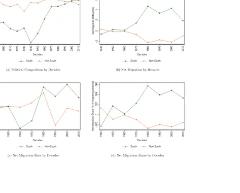
as a fraction of all migrating individuals in a given time period. Panel (b), (c) and (d) in

Figure 1 graphs these net migration measures over time using the Census data. We plot net

migration for Southern states and non-Southern states separately and show that post-1960

there was a substantial shift in internal migration patterns in the US: away from other states

and into the South. We can also see this in Panel C of Table 1, where net migration in the

Southern states went from being negative in decades pre-1960 to positive post-1960. This

pattern reverses the trend observed in the earlier part of the century reported in Wright

(1987 (Table 2); and 1999 (Table 1)) where there was mass exodus from the Southern states.

We argue and go on to show that one key reason for these shifts in migration patterns was

due to changes in political competition in the US South relative to the non-South throughout

the century.

Our measure of political competition follows Besleyet al. (2010) and uses data originating

set of directly elected state executive o¢ces.5 _{A competitive election is one where the}

result is close, accordingly, Besley et al. (2010) de…ne a party neutral measure of political

competition to be the following:

(27) P Cst = jdst 0:5j

Where P Cst is political competition in state s at time t and dst is the vote share of the Democrats in all state-wide races in state s at time t. Panel (a) of Figure 1 extends

the work of Besley et al. (2010) and plots 10-year averages of political competition over

time separately for Southern and non-Southern states. As can be seen, there is signi…cant

variation in political competition across states and over time. There are some noteworthy

trends to point out. First, there is a signi…cant di¤erence in the level of political competition

between Southern and non-Southern states. Second, this di¤erence increases between 1890

and 1940 due to a reduction in political competition in Southern states. Third, beginning in

1940s, there is an increase in political competition in the US South relative to the US

non-South to such a degree that, today, the US non-Southern states are more politically competitive

than non-Southern states. Panel C in Table 1 also shows the changing disparity in political

competition between Southern states and the rest of the US pre- and post-1960. Over

this period political competition in Southern states increased from an average of -0.197 (a

winning margin of about 70% to 30%) to -0.073 (a winning margin of about 51% to 49%).

As pointed out by Besley et al. (2010), amongst others, the …rst half of the 20th century

was characterized by the virtual monopoly of the Democratic Party in many of the Southern

states. By 1880s, the Democrats were …rmly in power in the Southern states. However,

because the US South had a large black (and low income) majority, white Democrats still

feared a possible resurgence of minorities and the poor at the polls. Accordingly, several

5_{These elections range from US representatives, over the governorship, to down-ballot o¢cers, such as}

voting restrictions including the white primary, multiple ballot boxes (e.g. South Carolina’s

"Eight Box Law" which was an indirect literacy test), poll taxes, literacy tests, and ultimately

violence were employed over the years to restrict minorities and the poor from voting. This

e¤ectively eliminated opposition to the Democrats during this period, and the fall in political

competition is clearly visible in Figure 1.

Over time, a number of these practices were eliminated, and by the late 1950s, the

remain-ing two major obstacles to full political participation were the poll tax and the literacy test.

It was not until the 1960s that the dominance of the Democrats in US South was challenged

with the Twenty-fourth Amendment to the U.S. Constitution, rati…ed in 1964, prohibiting

poll taxes in federal elections, and the introduction of the 1965 Voting Rights Act which did

two things: (1) it authorized the US attorney general to challenge the constitutionality of

the use of poll taxes in state and local actions; and (2) it provided for direct federal action in

"covered jurisdictions" to prohibit the use of the literacy test.6 _{Consequently, federal courts}

quickly struck down the remaining poll taxes in Alabama, Mississippi, Texas, and Virginia.7

The 1965 Voting Rights Act also targeted the states of Georgia, Louisiana, Mississippi, South

Carolina, Virginia, 40 counties in North Carolina, Apache County in Arizona, and Honolulu

County in Hawaii because of their literacy tests and low turnout. The resultant impact on

political competition in the US South was a reversal of the pre-war decline. Wright (1987

pg. 173) sums up the transformation of Southern politics during this period nicely:

"To the economic historian taking a view of the South and its political

econ-omy in the broadest sense, it appears that a more fundamental transformation

was underway, a basic change in the priorities of the region’s economic interest

groups"

Before moving onto to our main analysis, we …rst perform a simple di¤erence-in-di¤erence

6_{A covered jurisdiction was de…ned to be a state, county, parish, or town that used a test or device (e.g.,}

a literacy test) and had less than a 50 percent turnout in the 1964 presidential election.

analysis of our key variable of interest P Cst as well as our measures of net migration. Our treatment group is all States for which the 1965 Voting Rights Act targeted (i.e. Alabama,

Georgia, Louisiana, Mississippi, South Carolina, Virginia, North Carolina, Arizona, and

Texas). The baseline period is dates prior to 1965 and the follow up period is dates after

1965.8 _{The results for the univariate analysis are presented in Panel A of Table 2 and the}

multivariate version where we control for time and state …xed e¤ects are reported in Panel B.

For all four variables, the di¤erence-in-di¤erence statistic is positive and signi…cant which

suggests that political competition in the Southern states increased signi…cantly relative to

all other states after the introduction of the Voting Rights Act in 1965. This same result

was also found for our measures of net migration.

4

Empirical Approach & Results

We will discuss our empirical strategy in two steps, our approach di¤ers slightly depending

on the migration data that we employ. First, we discuss our approach using Census data

covering the period 1940-2010. Second, we discuss our empirical approach using the more

recent IRS annual migration data.

The spirit of our model is to capture long term shifts in political competition and the

resultant impact on migratory choices. Using the Census data, we are considering migratory

choices over a longer time period (data are decennial) in response to longer-term changes in

political competition and other economic variables. Accordingly, the analysis here can be

considered as our main results. Proposition 2 states that higher political competition leads

to higher inward migration (positive net migration). To test this empirically, we estimate

regressions of the form:

(28) N Mst = s+ t+P Cst+

0

X+"st,

8_{Note that we are using 10 year averages forP C}

where N Mst is the net migration in state s at timet. P Cst is political competition in state

s at time t, s and t are state and time …xed-e¤ects. X is a vector of state-speci…c,

time-varying economic and socio-demographic characteristics including: personal income

growth (Growth), taxation as a fraction of personal income (Tax), capital expenditure as a

fraction of taxes (Capital), the proportion of the population that is non-white (Non-white),

the proportion of the population over 25 with high school education (High School), and the

proportion of the population who are female (Female). Unconditional sample means for

these variables are contained in Table 1.9 We estimate robust standard errors adjusted for

clustering at the state level. We emphasize the long-term shifts in two ways: we instrument

for political competition (see below), and average the data over longer periods. Since net

migration …gures are obtained from the Decennial Census, we only have an observation every

decade. Accordingly, P Cst and all controls are averaged over the 10 year period leading up to the decade in question. For example, the …gure for P Cst in, say, 1960 is the average of the variable from 1951 to 1960. The results are robust to the period chosen to average over

as well as using end of decade …gures rather than averaging.

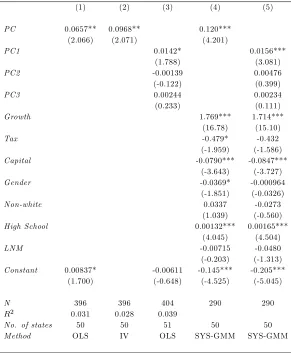
Tables 3, 4 and 5 present the results for our di¤erent measures of net migration: net

migration, net migration rate, and net migration share respectively. In each table, column

(1) is an estimation of (28) without control variables contained in X. The second column

of results addresses the possibility of reverse causation from net migration to the degree of

political competition (indeed, we argue there is reverse causation in Proposition 3). To

min-imize such endogeneity, which would likely bias our estimates downwards (since Proposition

3 argues that negative net migration leads to an increase in political competition), we use the

exogenous intervention of the federal government in the Southern states via the 1965 Voting

Rights Act to instrument for political competition.10 _{Speci…cally, we instrument political}

competition with a variable which is equal one after 1965 if a state was the target of federal

9_{State personal income is available from the Bureau of Economic Analysis for the period after 1929. Tax}

intervention due to having either a literacy test or a poll tax (or both) and zero before 1965.

In column (3) we follow Besley et al. (2010) and create binary indicators for high,

medium and low competition and include these, rather than the continuous measure of

political competition. These indicators correspond to values of political competition larger

than -0.10 (PC1), -0.25 (PC2), and -0.4 (PC3) respectively.11 _{Finally, columns (4) and (5)}

repeat the analysis in columns (2) and (3) respectively with our additional control variables

as well as lagged net migration (LNM). Since we include …xed-e¤ects as well as a lagged

dependent variable, we report results from System-GMM (Arellano and Bond, 1991; Arellano

and Bover, 1995; Blundell and Bond, 1998) estimation (rather than IV or least squares).

A consistent picture emerges across all three tables. Political competition is positively

related to net migration. That is, we …nd strong support for Proposition 2 which states that

an increase in political competition will lead to positive net migration, even after controlling

for other factors.

To be consistent with existing studies of net migration, we focus the rest of our discussion

on Table 4 where our dependent variable is the state net migration rate (net migration

as a proportion of state population). Comparing column (1) with (2) we see that OLS

estimates do in fact underestimate the impact of competition on net migration. When we

include additional control variables in column (4), the coe¢cient on political competition

increases. Columns (3) and (5) show that the e¤ect of political competition indeed appears

to be nonlinear - it seems that net migration only responds to greater competition when

competition exceeds -0.10.

Our results are not only statistically signi…cant but also economically signi…cant. Our

coe¢cient estimates range from a conservative 0.07 in column (1) to 0.12 in column (4). This

suggests that an increase in political competition by about 0.3 - typical for many Southern

states over the last century - will lead to an increase in the net migration rate of between 0.021

(or 21 individuals per 1000 population) and 0.036 (or 36 individuals per 1000 population).

11_{Note the interpretation, for example, the estimated e¤ect of a change in political competition from below}

To help put this in context, annual birth rates in the US over a similar period have declined

from just over 30 births per 1000 population in 1910 to less than 14 per 1000 population

by 2010.12 _{These …gures are not directly comparable since birth rates are annual and the}

migration numbers are …ve-year migration rates, so to help with comparison, if we take the

1910 and 2010 birth rates as upper and lower bounds respectively, then 5-year birth rates are

somewhere between 150 per 1000 population and 70 per 1000 population. Our estimation

suggests that the impact of increasing political competition on net migration go quite some

way to arresting the impact of declining birth rates on (Southern) state economies.

Looking at the other results from our main regression with controls (column 4) there

does not seem to be much controversy. As expected, higher income growth and a larger

proportion of the state that has high school education is positively related to net migration,

while higher taxes as a proportion of income is negatively related to net migration. There is

evidence to suggest that higher capital expenditure relative to taxes is negatively related net

migration, while at …rst this seems counterintuitive, this may simply re‡ect that high capital

expenditure is correlated with larger governments, which impose higher taxes. There is no

relation between the proportion of non-whites in the population and net migration while

the proportion of females is negatively related (we do not have an a priori expectation as to

why this may be). Finally, surprisingly, past net migration does not seem to be related to

current migration.

We reestimate (28) using annual migration data from the IRS. During the IRS sample

period of 1988-2010, there is signi…cantly less variation (both across states and overtime) in

political competition, the analysis here explains current state level variation in short-term

migratory decisions in response to short-term changes in political competition. Since our

model emphasizes longer term shifts, we consider this analysis to be a robustness test to the

preceding results.

State elections are on a two year cycle, and we have annual migration data, accordingly,

we need to either (1) aggregate net migration over a two year window; or (2) follow Besley

et al. (2010) and interpolate our political competition variable in between elections. We do

both and the results are the same. We report results using migration aggregated over two

years as these are our conservative estimates. The …nal decision we need to make is whether

we calculate net migration based on the number of …lers (which approximates households)

or exempt individuals (which approximates people). We choose the former to provide the

most conservative estimate of net migration.

The drawback using this second data set is that we cannot look at longer term trends

and we cannot adequately control for the potential of endogeneity using the introduction of

the Voting Rights Act to instrument for political competition (we do however treat political

competition as an endogenous variable in the System-GMM estimation). A bene…t, however,

is we are able to control for additional political variables of interest that may also explain

migration patterns.

In this analysis our vectorXof state-speci…c, time-varying economic and socio-demographic

characteristics include: Growth, Capital and Tax, which are de…ned in the same way as

be-fore, the percentage of high school dropouts (Dropout), the proportion of blacks (Black),

and the proportion of female-headed households (Female), and the proportion of employed

individuals (Employed).13 _{In addition, to investigate whether our results are indeed due to}

changes in political competition rather than di¤erences between the Democratic and

Repub-lican Party, we follow Besley et al. (2010) and use an indicator variable of the governor’s

party a¢liation (Democrat) equal to one if the governor is a Democrat, equal to zero if he

is a Republican, and missing in the case of Independents.14 _{To measure state-level party}

composition or control (Control), we use the fraction of Democrat incumbents: D=(D+R)

less the fraction of Republican incumbentsR=(D+R)in all statewide races (excluding the president).15

13_{Employment is from Bureau of Economic Analysis. Demographic variables are taken from Beck, Levine}

and Levkov (2012) and originally sourced from the Bureau of Labor Statistics.

14_{This information was obtained from the National Governors Association at www.nga.org.}

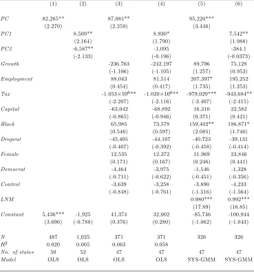
Tables 6, 7 and 8 present the results for our di¤erent measures of net migration: net

migration, net migration rate, and net migration share respectively. In each table there are

six columns: without controls or lagged net migration (column 1), with controls but without

lagged migration (column 3), with controls and lagged migration (column 5), and columns

(2), (4) and (6) repeat the analysis in columns (1), (3) and (5) respectively replacing the

continuous measure of political competition with binary indicators for competition de…ned

previously.16

With few exceptions, our results are consistent with those using the Census migration

data. Again, focusing on the results for net migration rate (Table 7), our main regression

in column (5) reports an estimated coe¢cient of 0.01 or 1 household per 1000 population

(for a 0.1 increase in political competition - one third of the approximate 0.3 increase in

political competition in Southern states during the post-war period). Again, comparing

this to current approximate two-year birth rates of 28 per 1000 population the resultant

impact of political competition on net migration is not only statistically signi…cant but also

economically signi…cant - even in this later period when political competition across states is

much more homogeneous.17 _{Growth and lagged net migration are positively related to net}

migration as is the proportion of high school dropouts. The …rst two results just mentioned

are to be expected however the result suggesting that states with a higher dropout rate tends

to have positive net migration is puzzling, it may be the case that this result re‡ects the fact

that high dropout rates tend to be correlated with a less skilled labour force, implying that

there is a relatively higher demand for skilled labour in these states. Looking across the

tables, the only other consistent evidence we …nd is that higher taxes tend to be negatively

related to net migration.

supplied by James Snyder in electronic form.

16_{Note that due to the reduced variability in political competition in this sample period, we only use the}

…rst two indicators variables instead of all three.

17_{It is worth noting that the coe¤cient on political competition is positive but insigni…cant in colummn}

5

Concluding Remarks

We develop and test a model of political competition and migration. Our model predicts

that an increase in political competition (in one state relative to the other) leads to an

increase in net migration.

Our application uses the substantial variation in political competition across US states to

study its impact on net migration ‡ows. Using migration data from the Decennial Census

for the entire post-war period we show that political competition is positively related to net

migration. That is, people tend to migrate towards more politically competitive states. This

result is robust to speci…cation and estimation technique. Further, to alleviate endogeneity

concerns, we use the introduction of the 1965 Voting Rights Act to instrument for political

competition. Results remain unchanged.

In further tests, we use annual migration data from the IRS covering the last two decades

to investigate if the longer term relationship between political competition and migration is

still observed for a more recent period where there is signi…cantly less variation in political

competition across the states. We again …nd consistent evidence that political competition

is important for migratory choices. So to answer our original question: do individuals "vote

with their feet" in response to a lack of political competition? Yes.

REFERENCES

[1] Acemoglu, D. and J. Robinson (2000), "Why Did the West Extend the Franchise?

Democracy, Inequality, and Growth in Historical Perspective." Quarterly Journal of

Economics 115, 1167-1199.

[2] Ansolabehere, S. and J. M. Snyder Jr. (2002), "The Incumbency Advantage in U.S.

Elections: An Analysis of State and Federal O¢ces, 1942–2000."Election Law Journal,

[3] Arellano, M. and S. Bond (1991), "Some Tests of Speci…cation for Panel Data: Monte

Carlo Evidence and an Application to Employment Equations." Review of Economics

Studies 58, 277-297.

[4] Arellano, M. and O. Bover (1995), "Another Look at Instrumental Variable Estimation

of Error Component Models." Journal of Econometrics 68, 29-51.

[5] Baechler, J. (1976), The Origins of Capitalism, translated by Barr Cooper, Oxford:

Blackwell.

[6] Banzhaf, H. S. and R. P. Walsh (2008), "Do People Vote with Their Feet? An Empirical

Test of Tiebout’s Mechanism." American Economic Review 98, 843-863.

[7] Beck, T., R. Levine, and A. Levkov (2012), "Big Bad Banks? The Winners and Losers

from Bank Deregulation in the United States" forthcoming in the Journal of Finance.

[8] Besley, T., T. Persson and D. M. Sturm (2010), "Political Competition, Policy and

Growth: Theory and Evidence from the US." Review of Economics Studies 77,

1329-1352.

[9] Blundell, R. and S. Bond (1998), "Initial Conditions and Moment Restrictions in

Dy-namic Panel Models." Journal of Econometrics 87, 115-143.

[10] Ferrie, J. P. (2003) "Internal Migration." In Historical Statistics of the United States,

Earliest Times to the Present: Millennial Edition, Ed. S. B. Carter, S. S. Gartner, M.

R. Haines, A. L. Olmstead, R. Sutch, and G. Wright, 1st vol., pp. 489–94. New York:

Cambridge University Press.

[11] Greenwood, M. J. (1975), "Research on Internal Migration in the United States: A

Survey." Journal of Economic Literature 13, 397-433.

[13] Greenwood, M. J. (1997) “Internal Migration in Developed Countries.” In Handbook of

Population and Family Economics, Ed. M. R. Rosenzweid and O. Stark, 647-720. New

York: Elsevier Science, North-Holland.

[14] Husted, T. A. and L. W. Kenny (1997), "The E¤ect of the Expansion of the Voting

Franchise on the Size of Government." Journal of Political Economy 105, 54-82.

[15] Krugman, P. (1995),Development, Geography, and Economic Theory. Cambridge: MIT

Press.

[16] Li, K. and R. Smyth (2004), "Division of Labour, Specialization and the Enforcement

of a System of Property Rights: A General Equilibrium Analysis." Paci…c Economic

Review 9, 307-326.

[17] Liu, W.-M. and X. Yang (2007), “E¤ects of Political Monopoly on Economic

Develop-ment”, Paci…c Economic Reviews 12, 69-78.

[18] Molly R., C. L. Smith, A. Wozniak (2011), "Internal Migration in the United States."

Journal of Economic Perspectives 25, 173-196.

[19] North, D. C. and B. R. Weingast (1989), "Constitutions and Commitment: The

Evolu-tion of InstituEvolu-tional Governing Public Choice in Seventeenth-Century England."

Jour-nal of Economic History 49, 803-832.

[20] Polo, M. (1998), "Electoral Competition and Political Rents”, Mimeo, IGIER, Bocconi

University.

[21] Rosenbloom, J. L., and W. A. Sundstrom (2004), "The Decline and Rise of Interstate

Migration in the United States: Evidence from the IPUMS, 1850–1990." InResearch in

Economic History, Vol. 22, Ed. Alexander Field, 289-325. Amsterdam and San Diego:

[22] Sachs, .J, W. T. Woo, and X. Yang (2000), "Economic Reforms and Constitutional

Transition." Annals of Economics and Finance 1, 423-479.

[23] Saks, R. E. and A. Wozniak (2011), "Labor Reallocation over the Business Cycle: New

Evidence from Internal Migration" Journal of Labour Economics 29, 697-739.

[24] Svensson, J. (1998), "Controlling Spending: Electoral Competition, Polarization, and

Primary Elections", Mimeo, The World Bank.

[25] Tiebout C. M. (1956), "A Pure Theory of Local Expenditures." Journal of Political

Economy 64, 416-24.

[26] Wen, M. (1998), “An Analytical Framework of Consumer-Producers, Economies of

Spe-cialisation and Transaction Costs.” In: Increasing Returns and Economic Analysis,

edited by K. Arrow, Y-K. Ng and X. Yang, London: Macmillan.

[27] Wright, G. (1987), “The Economic Revolution in the South”, Journal of Economic

Perspectives 1, 161-178.

[28] Wright, G. (1999), “The Civil Rights Revolution as Economic History”, Journal of

Economic History 59, 267-289.

[29] Yang, X. and Y.-K. Ng (1993),Specialization and Economic Organization, a New

Clas-sical Microeconomic Framework. Amsterdam: North-Holland.

[30] Yang, X. and W.-M. Liu, (2009),Inframarginal Economics. Singapore: World Scienti…c.

[31] Yao, S. (2002a), "Privilege and Corruption: The Problems of China’s Socialist Market

Economy." American Journal of Economics and Sociology 61, 279-299.

[32] Yao, S (2002b), "Walrasian Equilibrium Computation, Network Formation, and the

[33] Young, A. (1928), "Increasing Returns and Economic Progress." Economic Journal 38,

A

Appendix (Proofs of Propositions)

Proof of Proposition 1. To prove the inverse relation between political competitiveness and

tax, we di¤erentiate t with respect to :

(29) dt

d = 1 n 1

n

n 1 (n)<0:

Since is positively related to the state’s political competitiveness, states with a lower level

of political competitiveness will have a higher equilibrium tax rate.

Next we prove that states with a lower level of political competitiveness will have

in-ferior economic performance. To prove this statement, it is su¢cient to show that the

equilibrium level of division of labor n increases with , as n is positively related to the degree of commercialization, market integration, trade dependence, production

concentra-tion, occupation diversity, and the extent to which the endogenous comparative

advan-tage is utilized. De…ne G lnug(n( ); ) = h(n) + nln[1 n11 (n)], where h(n) =

mln[1 b a(m n)] +nln [1 a(m n+ 1)] (m+n) lnm+nln(n 1) +nlnn. The …rst order condition in (25) is equivalent to:

(30) @G

@n =h

0

(n) + n

1

n 1

1 n11 (n)

ln

(n 1)2 (n)

0

(n) + ln[1 n11 (n)] = 0:

Di¤erentiating (30) again (with respect ton and ) and using the implicit function theorem, it can be shown that:

(31) dn

d =

>0

z }| {

@2G=@ @n @2G=@n2

| {z }

<0

>0:

@2_{G=@ @n:}

(32) @

2_G

@ @n =

n+2

n 1

(n 1)(1 n11 (n))

"

n 1 n11 (n)

ln

(n 1)2 (n)

0

(n) + (n) n 1

#

.

It can be easily seen that @2_{G=@ @n >0 because for the …rst order condition (30) to hold,} ln

(n 1)2 (n) 0

(n)must be positive sinceln[1 n11 (n)] = lnt <0. Expression (31) implies

that as the degree of intolerance decreases, the state becomes less politically competitive

(more rent extraction), the equilibrium level of division of labor, n, decreases, and thus lowers economic performance. Q.E.D.

Proof of Proposition 2. Suppose there is a positive exogenous shock to the level of political

competitiveness in state 1. For example, an extension of voting rights in state 1 raises 1

to 0

1. If the revised constraint is binding, uy;1 will increase to u0y;1 due to the result of

proposition 1; when rises, the tax rate falls and the level of division of labor increases. The

real per capita income of commoners in state 1, uy;1, increases. Meanwhile, if the impact of

the shock is su¢ciently high, the non-migration constraint for commoners in state 2 may be

violated:

(33) uy;2 <maxf 2; u

0

y;1g.

State 2’s commoners will move from state 2 to state 1. As the population in state 1, M1,

increases, the scope for further specialization and division of labor increases, which implies

that the total number of consumer goods will increase. For example, if the state consists

of two individuals, the maximum number of consumer goods is two when both are fully

specialized. When the population increases to three, the maximum number of consumer

goods increases to three. Because of the preference for diverse consumption (see (1)), the

Proof of Proposition 3. If the impact of the positive shock to 1 is su¢ciently high, state 2’s

commoners will move from state 2 to state 1. The population in state 2, M2, tends to zero

and the population in state 1 tends to M. Since the utility of the ruling elite increases as the population size increases (more tax revenue), and asM2 tends to 0, their utility goes to

zero. As both states compete and undercut (through lowering the tax rate), in equilibrium,

(34a) u0

y;1 = maxf

0

1; u

0

y;2g;

(34b) u0

y;2 = maxf 2; u0y;1g;

for u0

Table 1: Summary Statistics

This table reports the mean of variables that are used in the empirical analysis. Political competition (PC) data come from Ansolabehere and Snyder (2002) and the data covers the period from 1890 to 2010. Migration data come from two sources: (1) individial income tax returns …led with the IRS from 1988 through 2010, and (2) the US Census from 1940 through 2010. Net Migration is the net interstate migration - the number of individuals that migrate in less those who migrate out of a particular state. Net Migration Rate is the net migration as a proportion of the state population. Net Migration Share is the net migration as a fraction of all migrating individuals in a given time period. Growth is the income growth. Employment is total employed persons as a percentage of population. Tax is total tax collected as a percentage of total income. Capital is total capital expenditure as a percentage of taxes. Black is the percentage of black population. Dropout is total high school dropouts as a percentage of population. Democrat is a dummy variable that equals 1 if the Governor is a Democrat.

Control the fraction of Democrat incumbents less the fraction of Republican incumbents in

all statewide races (excluding the president). Female is the percentage of female population.

Non-white is the percentage of non-white population. High School is the percentage of adults

(>25 years old) with high school diploma.

PANEL A: Political Competition and Migration

1988-2010 1940-2010

Mid West

North

East South West

Mid West

North

East South West

PC -0.056 -0.080 -0.065 -0.077 -0.068 -0.071 -0.149 -0.069 Net migration 4161 11959 -9724 -2855 -0.521 -0.865 0.485 0.486 Net migration rate 0.001 0.000 -0.001 -0.002 -0.017 -0.005 0.001 0.018 Net migration share 0.002 0.005 -0.004 -0.001 -0.003 -0.005 0.002 0.003

PANEL B: Demographic and Economic Variables

1988-2010 1940-2010

Mid West

North

East South West

Mid West

North

East South West

Growth 0.061 0.052 0.061 0.069 0.044 0.047 0.051 0.063 Tax 0.063 0.063 0.065 0.071 0.052 0.051 0.059 0.061 Capital 0.169 0.158 0.178 0.196 0.260 0.268 0.270 0.312 Employment 0.609 0.582 0.553 0.590 - - -

-Black 0.067 0.063 0.188 0.026 - - -

-Dropout 0.072 0.085 0.126 0.086 - - - -Democrat 0.359 0.448 0.552 0.488 - - - -Control -0.017 0.168 0.046 -0.110 - - - -Female Head 0.338 0.392 0.369 0.343 - - -

-Female - - - - 0.520 0.522 0.562 0.510