A Nelson Winter Model of the German Economy

A Nelson-Winter Model of the German

Economy

Quaas, Georg

2 August 2012

Online at https://mpra.ub.uni-muenchen.de/40447/

Georg Quaas

1 The basic idea

A key feature of the class of models constructed on the basis of Nelson and Winter’s (1982) evolutionary theory is the coexistence of a micro- and macro-economic structural level that are connected by a simple aggregation procedure and by a more or less developed specification of a market mechanism. Theories of the household, firm, production process, banks and markets in which the researcher is interested have to be formulated mathematically and implemented in order to create a special version of the Nelson and Winter model. On the micro-economic level, as many firms and households are installed as the computer’s capacity and velocity can handle. Similar to what is done in theory, supply and demand are formulated separately. The modeled market structures function as intermediaries between the economic actors and while creating a structure that is summarized by macro-economic variables such as gross domestic product and average wages. A complete specified model can be run over a time-span for which real data are available. The aggregated results of the interactions of the actors and structures produce a time series of macro-economic variables that can be compared with the observed variables. Unlike the common econometric models of a national economy, a statistic estimation of key parameters plays no role and is replaced by an a priori setting of their values. However, as with econometric models, equations and their parameters are interpreted and treated as representations of causal relationships. Therefore dynamic solutions of a specific Nelson and Winter model with the goal to approximate the observed data is not only possible, but it is the only possibility of proving the a priori determination of the parameter values. The fit of the model to the real data can be used to adjust parameter values by adapting the model to the data. It serves as a measure of the correctness and goodness of the whole model and the theories that are corroborated by its structures.

2 Personal note

decided to try to come as close as possible to what we thought were the authors’ intentions. In fall 2006 we planned to advance the model after it was working. This was the case in February 2007—the model was implemented on the empirical base of yearly data of the German economy from 1970 to 2004 and produced results similar to what Nelson and Winter reported. The development has not been continued, but the model was used for demonstration purposes for the author in his teaching. Expecting a growing interest in alternatives to so-called mainstream theories, a new launch of the research must begin with a documentation of the results achieved previously by the former implementation of the model.

3 The overall structure

The modeled structure of a firm consists of several parts, a (rather truncated) formulation of the production process by means of an input-output matrix and the attached management structure comprising cost-control, the use of capital and profit, research and development, including decision rules for handling these processes. The next section presents a comprehensive description of the model. To date, there is no structure corroborating households in the model, because Nelson and Winter neglected this, too. The model depends on the observed numbers of earners as a proxy for the household members delegated to the labor market due to the offered wage rate. The labor market in the model consists of a simple wage setting equation. The formulation of the market of commodities and services reduces to a simple aggregation; in other words, it is assumed that commodities for investment are of the same nature as commodities for consumption. The output of firms is immediately a part of the gross domestic product. Therefore, the price of the output is set to one. The formulation of the capital market consists of an allocation rule and procedure for the unemployed capital that is given to potential firms with sufficiently high profit expectations. Currently, the model is not endowed with governmental structures such as taxes or subsidies.

4 The model of a firm

One of the key elements of Nelson and Winter’s model is the microeconomic structure of the firm—a partial model that is implemented as often as firms are supposed to exist in the modeled economy. The structure of an enterprise can be depicted only in a very abstract way, but it is not the purpose of the N&W model to map any real enterprise, in spite of the fact that this could be achieved if the necessary data were available.

output is immediately part of the GDP. In other words, there is no market for services and goods implemented. On the other hand, because GDP is the only product of the economy, it must serve as a means of production and consumption. The connection between the interior structure of a firm, its input and output and its influence on the GDP is described by the following passage:

“The model involves a number of firms, all producing the same homogeneous product (GNP)1, by employing two factors: labor and physical capital. In a particular time period, a firm is characterized by the production technique it is using—described by a pair of input coefficients

(

)

The following definitions are the same for every firm implemented in the model and for every particular period of time.

4.1 The production process

The technological structure of the production process of the i-th firm and its production technique are characterized by a pair of input coefficients that refer to the spent physical capital and to the applied and paid labor. Both are put together in one column vector:

ci i

li

a Capital

A

a Labor

⎡ ⎤ ⎡ =_{⎢ ⎥ ⎢}=

⎣ ⎦ ⎣ ⎦

⎤ ⎥

(1)

The coefficients are interpreted (i) as the amount of investment goods used to produce one unit of the firm’s physical output and (ii) as the amount of labor applied in the same production process measured in hours, for instance.

Normally, the amount of capital used in a production process includes the depreciation of the applied capital stock and the amount of those goods and services that are the result of other firms’ current production and that are totally consumed by the i-th firm’s production process in a given period. This “normal” interpretation of used capital can be (and has to be) changed if required by the needs of a special architecture of the model. For a simple version of the model, we can dispense with the inclusion of the intermediate inputs.

1

The difference between gross national and gross domestic product is negligible in the framework of a simple model.

2

4.2 Accounting

Nelson and Winter mention prices assigned to the inputs; one of them shall be set to one (210). I take this as an inducement for the introduction of the prices of capital and of labor. Let:

0 0 c l p P p ⎡ = ⎢ ⎣ ⎦ ⎤

⎥ (2)

be the price-matrix with referring to the price of one unit of a pile of capital goods (thought to be homogeneous) that is measured empirically with the help of corresponding indices, and refers to the wage per working hour (wage rate) symbolized by W in the original text. According to Nelson and Winter, the numerical value of is set to 1 and the wage rate

c p

l p

c

p p_l =W depends on the

demand of labor (214). Therefore we can specify the price-matrix with:

0 1 0

0 0 c l p P p W ⎡ ⎤ ⎡ =_{⎢ ⎥ ⎢}= ⎣ ⎦ ⎣ ⎦ ⎤

⎥. (2’)

The i-th firm’s output shall be defined by (213) as the value of the part of GDP that is produced by firm i. Physically, Q consists of the means of consumption and means of production. Since households are not modeled at the moment, only the use of the GDP as means of production is relevant. However, the composition of the output will play a role when the market for goods and services and prices of capital and consumption goods are used in the further development of the model.

i Q

If we divide by its price , we get the output in real or physical terms, i.e., the number of as homogeneous supposed goods

i

Q p_c

i c

Q p that are produced by the

i-th firm. Because is set to 1, numerically denotes the real output and its value expressed in current prices. For the further development of the model the differentiation between nominal output (at current prices) and real output (at constant prices) can become important.

c

p Q_i

The i-th firm’s consumption of capital goods and its use of labor forces depend on its production level during the regarded period. It is measured by the column vector:

ci ci i c

i

li li i c

n a Q p

N

n a Q p

⎡ ⎤ ⎡ ⎤ =_{⎢ ⎥ ⎢}= _⎥ =

In other words: The technological structure has to be multiplied by the total amount of the i-th firm’s physical output to get its consumption of capital goods and total application of labor. Both are components of the demand-vector, symbolized by N_i. One of its components, n_li, equals the amount of labor L_i

employed by the firm during the production period, i.e.,

i li i c

L =a Q p . (4)

Let be the total cost of i-th firm’s total production. Now its amount can be computed easily with the help of the sum-vector

i C

[ ]

E=

as follows: the i-th firm’s costs are its priced (multiplied by prices) consumption of capital goods and its priced amount of applied labor summed up by E:

i i i i c ci i l li i c ci i i

C =EPN =EPA Q p =a Q + p a Q p =a Q +WL . (5)

According to Nelson and Winter, a firm is characterized by its applied capital stock K_i, among other factors. We interpret K_i as the value of a purposefully arranged physical pile of capital goods that embodies the firm i physically. Conditioned by its application for production purposes and by purchases of new compounds, machinery, tools, etc., the capital stock changes over time. Let be the value of the part of the i-th firms capital stock that is consumed during the production period and

i D

i

IB the value of newly bought capital goods, i.e., the gross investment of capital goods. Then, the changing value of the capital stock can be jot down as follows:

(

)

( )

( )

( )

i i i i

K t+ = K t −D t +IB t

i

. (6)

Nelson and Winter suppose that depreciation, , is caused by a random mechanism. “…each unit of capital is, independently, subject to a failure probability of … 0.04 each period” (213). I interpret the effects of the decay-process purely deterministically as follows:

i D

0.04

i

D = ⋅K , (7)

i.e., the capital stock of the i-th firm is reduced by 4 percent at the end of a production period caused by “productive consumption” (Marx).

Although only part of the capital stock is consumed by the production process, the whole capital stock has to be applied. “A firm’s production decision rule is simply to use all of its capacity to produce output, using its current technique— no slow down or shut down is allowed for” (209).

If we ignore the (productive) consumption of capital goods and services stemming from the current production of other firms (“intermediate products”), Nelson and Winter’s production rule has the following consequences:

(i) The production of a given amount of output needs to consume a determined amount of capital goods according to formula (3):

i Q

ci i c ci

a Q p =n . (3’)

Following that decision rule, this amount cannot be more or less than the amount of depreciation a firm’s capital stock is allowing for, that is:

0.04

ci i c ci i i

a Q = p n = D = ⋅K (during a particular period t). (8)

To put it another way, the value of the output is determined by the technological structure, capital stock and its inherent depreciation rate:

1

0.04 i ci

Q =a− ⋅ ⋅K_i. (8’)

(ii) Another consequence of the production decision rule and depreciation rule is this:

(

) ( )

( )

( 1) 1 0.04

i i

K t+ = − K t +IB t . (6’)

After starting with a random distribution of total capital to all firms with sufficient high expected returns, their future endowment equals the remaining capital stock and additional gross investment into capital goods. “The capital stock, thus reduced [by depreciation or another ‘random mechanism’- G.Q.], is then increased by the firm’s gross investment in the period” (213).

Let us write this down step by step. The amount of wages that has to be paid in a period of time by the i-th firm is

1 _0.04 l

i i l li i c li ci i

c p

W L p a Q p a a K

p

−

= = ⋅ ⋅ . (9)

Referring to the “required dividends RK,” we interpret R as the interest rate. Then the total amount of dividends that the i-th firm has to pay to capital owners is RK_i, i.e., interest multiplied by the amount of applied capital.

Therefore, the amount of gross investment can be deduced as follows:

1

1 0.04

i l

i i l li i li ci

c c

Q p

i

IB Q p a RK a a R K

p p − ⎡⎛ ⎞ ⎤ = − − =_⎢⎜ − _⎟ ⋅ − ⎝ ⎠ ⎣ ⎦⎥ i

. (10)

Gross profit is supposed to be used for investment, i.e.,

i

K IB

π

Therefore the profit rate is given by

1

1 l _li 0.04 _ci c

p

a a

p

π

⎜ ⎟

⎝ ⎠ R. (12)

In the words of the authors, “The higher the value of R…the smaller the investment the firm is able to finance” (213).

(iii) Another approach to the complex of capital depreciation and investment goes as follows: the total output minus total cost minus dividends must equal the change of capital stock

i

Q C_i

i K :

(

)

( )

i i i i i i

K K t K t Q C RK

Δ = + − = − − . (13)

If we substitute C_i with the help of formula (5) and (8’) we get

1

1 0.0

i i ci i li i c i ci li ci i

c W

4

K Q a Q Wa Q p RK a a a R K

p

−

⎡⎛ ⎞ ⎤

Δ = − − − =_⎢⎜ − − _⎟ ⋅ − _⎥

⎝ ⎠

In the words of Nelson and Winter, “Thus, the next-period techniques of all firms are determined (probabilistically), and so are the next-period capital stocks” (214).

(iv) On the other hand, the change of capital stock according to (6) and (7) is:

( )

( )

( )

( )

i i i i i

K IB t D t IB t K t

Δ = − = − ⋅ . (14)

Equation (14) must be equal to (13’):

( )

( )

1

1 _{ci li ci} 0.04 _{i i} 0.0 _i c

W

a a a R K IB t K

p

−

⎡⎛ ⎞ ⎤

− − ⋅ − = − ⋅

⎢⎜ ⎟ ⎥

⎝ ⎠

⎣ ⎦ 4 t .

After eliminating identical terms, we get

( )

i li ci

c W

i

IB t a a R K

p

−

⎡⎛ ⎞ ⎤

=_⎢⎜ − _⎟ ⋅ −

⎝ ⎠

⎣ ⎦⎥ . (14’)

This result corresponds with Equation (10).

4.3 Research & Development

According to Nelson and Winter, research and development “activities of firms will be modeled in terms of a probability distribution for coming up with different new techniques” (210).

The technique of a firm is characterized by two components of the vector defined in Equation (1). Each of these coefficients is seen as a starting point of a randomly distributed new coefficient, which is (i) a result of R&D activities, and (ii) subject to an assessment procedure in which it has to be decided whether or not the set of new coefficients found in research and produced by development will be added to the production process (profitability check, p. 216).

Let the function frnd be a random number generator that produces random draws from a normal distribution with zero mean and unit variance. Furthermore, let

(

)

(

) (

)

a t = =a t = + ⋅s frnd

where s_i is the standard deviation of the corresponding technological coefficient. We assume that this standard deviation is constant and related to a specific firm. Because there is no assertion of the authors, one is free to choose one’s own rule.

In general, the vector A_i of the two technological coefficients of i-th firm’s production process could be changed after research and development have taken place according to the following formula:

(

)

(

)

( )

( )

1

1

ci c

ci ci

li l

li li

s frnd

a t a t

s frnd

a t a t

⋅ +

⎡ ⎤ ⎡ ⎤ ⎡

= +

⎢ ₊ ⎥ ⎢ _{⎥ ⎢ ⋅}

⎣ ⎦

⎣ ⎦ ⎣ ⎦

⎤

⎥. (15)

Here, I have assumed that two random generators are acting independently from each other. Nelson and Winter suppose that the two generators are connected in a special way (211-212) that allows making a difference between innovation concerning the coefficients of capital and labor consumption. This goal can be achieved more easily by a variation of the coefficients of the standard deviations above.

Another intention of Nelson and Winter is to differentiate between true innovation (inventions) and imitation. According to the authors, imitation is copying the technique of the largest firm (or of the most firms). They construe the probability functions that determine the implementation of a new (imitated or invented) technique. In addition, they allude to an alternative rule that is much more simple and, in my view, closer to reality. “An alternative rule turned up by the search process is adopted by the firm only if it promises to yield a higher return” (212).

That means: An assessment has to take place before adding a new technique to the firm’s infrastructure. In a nutshell, this assessment is a comparison of the production costs of the “old” with the “new” technique based on the current prices and current amount of GDP. In case the costs of the new production method are lower than the costs of the old ones, the new technique will be implemented as the technological base of the production process for the next period; however, the next period is ruled by changing prices and volumes unknown to the decision makers.

(

)

( )

(

)

( )

i i i i i c

C t + −C t = EP A t⎡_⎣ + −A t ⎤_⎦Q p <0. (16)

After a simple rewriting, we get the condition

0

ci c l c li l

s ⋅ frnd + p p ⋅ ⋅s frnd < (16’)

as the core of the decision rule for implementing a new technique. If (16’) is satisfied, the new technique will be applied by a firm; otherwise the old technique stays in place.

There is another decision rule that governs R&D activities. “Only those firms that make gross return on their capital less than the target level of 16 percent engage in search” ( 211) at all. The authors presuppose that “conservative firms” do not search at all if they are sufficiently profitable. This is an assumption that is designed to demonstrate that even an economy with lazy firms that do not maximize their profit produces macroeconomic patterns that can be captured by the neoclassical production function (227).

According to Equation (11), the sum of gross returns to capital is identical to the value of gross investment. If we divide (14’) by capital, we get the core of another decision rule for R&D activities:

1

1 _{li ci} 0.04 c

W

a a R

p

−

⎛ ⎞

− ⋅ − <

⎜ ⎟

⎝ ⎠ 0.16 . (17)

Taken all together, we have at least two hierarchical decision rules that control the implementation of the statistically generated sets of technological coefficients; there must be a sufficient low profit rate and an the expectation of a cost-reduction by the new technology in terms of the current prices.

5 The labor market

The prices of capital goods are set to one. The price of labor (measured in terms of hours) is the wage rate, and this function depends on the relationship between labor supply and demand. Nelson and Winter propose the following formula for the labor market:

(

)

c t

t

L

w a b

g

⎛ ⎞ ⎜ ⎟ = +

⎜ ₊ ⎟ ⎝ ⎠

The reader is free to choose the parameters a, b, g, and c. For the sake of simplicity, I set c=1 and g =0. It follows

( )

( )

W t = + ⋅a b L t or (18)

(

)

( )

(

)

( )

W t+ =W t +b L t⎡_⎣ + −L t ⎤_⎦ (18’)

as a very simple method to compute the next period’s wage rate.

6 Adjusting the model to the data

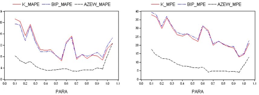
The appendix (Table 1) shows the results of an experiment comprising 20 tests. The first test starts with a parameter value of b=0.1, and for the next 19 tests this value is enhanced by 0.05 stepwise. The model runs 60 times in every test, and after that, it computes the averages of the produced time series and their standard deviations from the observed data. The key variables are the capital (K), the gross domestic product (BIP), the working time of earners (AZEW) and the wages per hour (W). Until then, all experiments showed that the standard deviation of wages was lowest at the smallest value of b. Therefore, I decided to use the other key variables as criteria for the best fit of the model. As can be seen in Figures 1 and 2, there are at least two local optimums of the mean absolute percentage error approximately at b=0.55 and between , and one optimum fit is located according to the mean percentage error at a parameter value of .

0.7...0.95 b=

0.95 b=

Fig. 1 & 2: Percentage errors of the model at different parameter values of b. Abbreviations: K = Capital; BIP = GDP; AZEW = working hours of earners in million; W = average wages per hour; MPE = mean percentage error; and MAPE = mean absolute percentage error.

observed data which are the product of the interplay between supply and demand, while the N-W-model treats them separately. Moreover, in our simple N&W model, the wage setting equation is the only mechanism that can steer the modeled economy against equilibrium. Therefore the values will probably get lower as more market structures are implemented.

7 Results

The Nelson-Winter model is driven by a random process; therefore, different runs will yield different results. Nevertheless, there are some general features that characterize the behavior of the model:

Fig. 3-6: Example of a run. Abbreviations: AZEW = working hours of earners in million; W = average wages per hour; A_L = input of labor per unit output (GDP); A_C = input of capital per unit output (GDP); _0 = baseline; _RS = difference between observed and fitted curve; _B = best firm (with the highest profit); Z = worst firm.

slightly below the observed data, because the capital-input coefficients are too low compared to the observed curve (Fig. 6).

(ii) Running the model shows the well-known events of a market economy: waxing and waning firms, some of them disappearing, giving way for newcomers with better profit-expectations. After 34 runs (years) a remarkable differentiation between small and big firms is the result (Fig. 7).

(iii) A short look at the table in the appendix shows that the error measures are too high for a prognostic use of the model. This is not surprising because there are important structures of an economy such as a market for goods and services that are missing in the implemented simple version of the Nelson-Winter model for the German economy.

Fig. 7. Random result of a run: The first 40 pillars refer to West German firms, the last 20 to East German firms. Missing pillars refer to disappeared firms, leaving their capital for potential enterprises with better profit expectations.

8 References

Appendix

Test‐#  PARA‐  K_MAPE  BIP_MAPE  AZEW_MAPE  W_MAPE 

  VALUE  MEAN  STDV  MEAN  STDV  MEAN  STDV  MEAN  STDV 

1   0.100   37.66   21.24   40.48   19.54   23.14   8.20   8.52   2.33 

2   0.150   39.24   20.38   41.28   19.05   20.02   6.44   10.84   2.64  3   0.200   30.97   15.29   32.02   13.65   16.40   5.52   12.73   3.76  4   0.250   30.56   19.39   31.33   18.70   15.69   6.24   15.63   5.11  5   0.300   30.09   13.94   30.56   13.08   14.49   4.48   17.19   4.91  6   0.350   27.42   10.35   27.27   9.78   13.23   3.74   18.77   4.89  7   0.400   27.99   10.28   27.11   9.77   11.75   3.14   18.62   5.07  8   0.450   29.04   10.45   27.39   9.87   10.67   3.18   18.58   5.42 

9   0.500   26.25   8.37   25.30   8.31   11.22   3.32   22.34   6.46  10   0.550   25.56   6.48   23.98   7.09   10.64   3.58   23.36   7.74  11   0.600   27.82   13.18   26.33   12.69   11.05   3.71   26.36   8.10  12   0.650   26.74   15.22   25.87   14.74   11.51   2.93   30.94   7.16  13   0.700   27.25   7.10   25.83   7.61   11.70   2.78   34.82   7.25  14   0.750   27.92   8.74   26.83   8.69   12.67   3.10   41.51   9.08 

15   0.800   31.19   7.33   30.19   8.06   14.64   3.24   50.91   10.18  16   0.850   33.23   8.48   32.98   8.65   16.20   3.13   59.82   10.65  17   0.900   34.51   8.31   34.08   9.51   16.90   3.98   68.40   14.62  18   0.950   36.53   6.71   36.20   7.60   18.92   3.50   82.63   15.81  19  1.000   40.17   10.92   41.30   11.90   23.67   8.35   107.98   32.86  20  1.050   44.49   12.83   45.46   14.54   27.84   12.71   131.19   51.63 

  PARA  K_MPE  BIP_MPE  AZEW_MPE  W_MPE 

Test‐#  VALUE  MEAN  STDV  MEAN  STDV  MEAN  STDV  MEAN  STDV 

1   0.100   39.41   37.84   34.31   39.55   0.06   17.61   0.02   6.09  2   0.150   45.63   36.51   41.90   37.58   4.21   14.21   2.18   7.36  3   0.200   28.14   29.88   22.65   31.10  ‐2.19   12.22  ‐1.51   8.44  4   0.250   22.89   36.20   18.31   36.94  ‐3.64   11.87  ‐3.14   10.25 

5   0.300   22.18   30.43   19.09   31.44  ‐2.25   10.57  ‐2.33   10.96  6   0.350   15.67   26.30   11.40   27.58  ‐4.36   8.79  ‐5.28   10.63  7   0.400   17.90   25.26   13.95   26.25  ‐3.13   7.73  ‐4.33   10.68  8   0.450   20.64   26.71   17.14   26.78  ‐1.72   7.54  ‐2.68   11.71  9   0.500   10.01   23.91   7.15   25.05  ‐4.27   6.91  ‐7.38   11.94  10   0.550   8.70   22.32   5.15   23.25  ‐4.32   6.58  ‐8.20   12.51  11   0.600   5.16   31.41   1.67   31.30  ‐5.24   7.04  ‐10.86   14.60 

12   0.650  ‐8.04   28.69  ‐10.56   28.07  ‐7.95   4.14  ‐17.85   9.30  13   0.700  ‐10.69   20.11  ‐12.34   20.84  ‐7.41   4.81  ‐17.93   11.64  14   0.750  ‐11.24   22.48  ‐13.80   22.16  ‐7.99   4.74  ‐20.70   12.28  15   0.800  ‐18.44   20.53  ‐20.68   20.69  ‐9.62   4.74  ‐26.59   13.11  16   0.850  ‐25.52   19.00  ‐27.62   19.25  ‐11.27   4.28  ‐33.08   12.58  17   0.900  ‐26.31   18.54  ‐28.00   19.31  ‐11.76   4.51  ‐36.58   14.03  18   0.950  ‐32.05   13.08  ‐33.41   13.53  ‐13.57   3.86  ‐44.52   12.66 

19  1.000  ‐37.14   14.59  ‐40.25   15.04  ‐17.92   8.20  ‐61.92   28.34  20  1.050  ‐39.03   21.39  ‐42.00   22.89  ‐21.39   13.02  ‐77.61   47.24