Munich Personal RePEc Archive
Sharing a polluted river network
Dong, Baomin and Ni, Debing and Wang, Yuntong
1 April 2012
Sharing a Polluted River Network
∗
Baomin Dong
School of Economics
Zhejiang University
Hangzhou, Zhejiang, China
Debing Ni
School of Management
University of Electronic Science and Technology of China
Chengdu, Sichuan, China
Yuntong Wang
†Department of Economics
University of Windsor
Windsor, Ontario, Canada
April 16, 2012
∗We thank the two anonymous referees and the associate editor Hassan Benchekroun
for their very helpful comments and suggestions that improve greatly our paper. We are grateful to Meidan Sun for her assistance in Section 3.4 of the paper. Wang would like to thank Peter Townley, Sang-Chul Suh, and Ronald Meng for the comments and suggestions. Wang’s research was supported by the SSHRC of Canada under grant # 410-2005-0620.
†Corresponding author. Tel: (519) 253-3000 ext.2382; Fax: (519) 973-7096; E-mail:
ABSTRACT: A polluted river network is populated with agents (e.g., firms, villages, municipalities, or countries) located upstream and down-stream. This river network must be cleaned, the costs of which must be shared among the agents. We model this problem as a cost sharing prob-lem on a tree network. Based on the two theories in international disputes, namely the Absolute Territorial Sovereignty (ATS) and the Unlimitted Ter-ritorial Integrity (UTI), we propose three different cost sharing methods for the problem. They are theLocal Responsibility Sharing (LRS), theUpstream Equal Sharing (UES), and the Downstream Equal Sharing (DES), respec-tively. The LRS and the UES generalize Ni and Wang (“Sharing a polluted river”, Games Econ. Behav., 60 (2007), 176-186) but the DES is new. The DES is based on a new interpretation of the UTI. We provide axiomatic char-acterizations for the three methods. We also show that they coincide with the Shapley values of the three different games that can be defined for the problem. Moreover, we show that they are in the cores of the three games, respectively. Our methods can shed light on pollution abatement of a river network with multiple sovereignties.
JEL classification: C71, D61, D62.
1
Introduction
Since ancient times, control of water resources has been the cause of many wars and conflicts. Accounting for more than 50% of the land area of the Earth, more than 200 river basins are shared by two or more sovereign na-tions. Unfortunately, the majority of this invaluable resource is polluted. One example is the Ganges-Brahmaputra basin, an international river basin shared by India, Bangladesh and Nepal. The Great Lakes is another exam-ple, consisting of a group of five1 large lakes in North America and shared
by Canada and the United States. In many of these shared waters, pollu-tion has become an increasing threat. To deal with this issue, internapollu-tional cooperation is needed.
Thus far, the studies on international waters have been focusing on water sharing. To name a few, they include Barrett (1994), Kilgour and Dinar (1996, 2001), Ambec and Sprumont (2002), Ambec (2008), Ambec and Ehlers (2008a,b), Ansink and Ruijs (2008), Marchiori (2010), and Wang (2011). Recently, there have been a number of papers considering the water pollution problem. Examples include Weber (2001), Hung and Shaw (2005), Ni and Wang (2007).
This paper considers the cost sharing problem of a polluted river network.2
Suppose that a number of agents (e.g., firms, villages, municipalities, or coun-tries) are connected in a river network. Some agents are located upstream and some downstream. In using the river network, agents may generate pol-lutants such as industrial chemicals, pesticides from agricultural run-off, or sewage. Consequently, a cost is incurred to each link of the network. These costs can be the costs that the agents must spend in order to clean up the polluted water to meet certain environmental standards. Or they can be the costs needed to maintain the water quality of the river network. Whatever these costs might be, they must be shared among the agents.
While it is clear that all the agents in the polluted river network should share the costs of cleaning up the network since these costs are incurred by their joint uses (or abuses) of the river network, it is not immediately clear how to assign these costs to each individual agent. While, the rights to use the
1
Many people argue that there are six by adding Lake St. Clair. 2
river come with responsibilities and responsibilities should be in proportion3
to their rights (uses) of the network, it is often hard if not impossible to identify precisely how much each agent uses the network and thus contributes to the pollution. Even these agents’ pollutant emissions can be identified, the complex interactions (e.g. chemical reactions) of the pollutants in flowing water make it difficult to estimate their actual impacts on pollution costs.
In the simplest two-agent case (i.e., one upstream and one downstream), when property rights on water are clearly assigned and the upstream agent’s pollutant emission is clearly identified, the Coase theorem (Coase, 1960) implies that the two agents can always resolve their problem through bilat-eral bargaining. In practice, however, most problems involve more than two agents. Moreover, property rights on most international river systems are not well-defined. For instance, in an international river system, downstream countries may argue that even the upstream countries can do whatever they want to the water they control but they shouldn’t alter the nature of the river system to the disadvantage of the downstream countries.4 However,
it is not clear or a simple matter to determine to what extent these rights actually mean for the water pollution problem. Therefore, it would be much more difficult to reach an agreement through multilateral bargaining.
To deal with this challenge, we focus on the problem of what a fair al-location of the pollution costs should be.5 We base our theory on the two well-known theories in international disputes. They are the theory of Ab-solute Territorial Sovereignty (ATS) and the theory ofUnlimited Territorial Integrity (UTI).6 In fact, Ambec and Sprumont (2002) have applied these
two theories in a water sharing problem. Later, Ni and Wang (2007) use them in a water pollution sharing problem. Our model differs from Ni and Wang (2007) in two respects. First, we consider a more general tree network
3
Aristotle said that equals should be treated equally and unequals unequally in pro-portion to their inequality.
4
See the Unlimited Territorial Integrity theory below. 5
We ignore the strategic reactions of the agents under a given allocation of the pollution costs, which will affect their polluting behavior and then the actual costs. We do not deal with the efficiency issue of a cost sharing method in our current model.
6
than their line-tree model. Second, we propose two different but equally compelling interpretations of the UTI theory. We show that these two differ-ent interpretations lead to two differ-entirely differdiffer-ent cost sharing methods. More importantly, the new interpretation of the UTI opens door to explore new cost sharing methods.7
Unlike in the water sharing problem, these two theories, each stand alone or together, still allow a lot of flexibility in choosing cost sharing methods in our polluted river network problem. In Ni and Wang (2007), the UTI is interpreted as a downstream responsibility (DR) principle which says that an agent is responsible for the cost of cleaning her own link and partially responsible for the costs of all her downstream links. In our model, we propose another interpretation of the UTI, which is exactly the opposite of the above DR principle. That is, the UTI can also imply that an agent is responsible for the cost of her own link and also partially responsible for the costs of all her upstream links. We call it the Upstream Responsibility principle (UR).8
To justify this alternative interpretation, revisit the water sharing prob-lem of Ambec and Sprumont (2002). It is shown that the combination of the ATS and the UTI determines a unique water sharing method called the Downstream Incremental Distribution method (DID). Ambec and Sprumont show that the DID method lexicographically maximizes the welfare of the agents according to the ordering from downstream to upstream. Thus, in a DID distribution the last downstream agent obtains the highest welfare she can possibly achieve, and then follows by the next to the last, and so on. If responsibilities should be in proportion to rights in any problem of distributive justice, then the UTI theory also implies that the downstream agents should bear some of the upstream costs of the network. To say it more directly, since they have benefited from being downstream agents in the water sharing problem, it is compelling to require them to pay part of the upstream environmental costs.9 In hindsight, downstream agents have
7
See the Concluding Remarks Section on the potential directions of research. 8
In fact, between these two opposing interpretations, a range of them can be proposed. For more on this, see Wang (2011) and the Concluding Remarks Section.
9
certain derivedupstream responsibilities.
Accordingly, we propose three different cost sharing methods for the prob-lem. The Local Responsibility Sharing (LRS) method, which corresponds to the Local Responsibility principle implied by the ATS, assigns costs to agents based on the costs that are associated with their locations. The Upstream Equal Sharing (UES) method,10 which corresponds to the Downstream
Re-sponsibility (DR) principle implied by the UTI, assigns costs to agents based on their associated local costs plus the equal sharing of their downstream costs. The Downstream Equal Sharing (DES) method is first introduced in this paper. It corresponds to the Upstream Responsibility principle implied by the UTI. The DES method assigns to each agent the associated local cost plus the equal sharing of her upstream costs.
The above three methods are axiomatized, respectively. In Theorem 1, the Local Responsibility Sharing method is characterized by the axioms of
Additivity, No Blind Costs, and Efficiency. In Theorem 2, the Upstream Equal Sharing method is characterized by the axioms of Additivity, Inde-pendence of Upstream Costs, Upstream Symmetry, IndeInde-pendence of Irrele-vant Costs, and Efficiency. In Theorem 3, the Downstream Equal Sharing method is characterized by the axioms ofAdditivity, Independence of Down-stream Costs, DownDown-stream Symmetry, Independence of Irrelevant Costs, and
Efficiency.
In the characterizations of the three methods, two axioms stand out. Additivity is an axiom used in all three characterizations. The Independence of Irrelevant Costs axiom is a new axiom we introduce in this paper and used in two of the three characterizations (the UES and the DES). As is well-known in the cost sharing literature, Additivity is a classical axiom (Shapley, 1953; Moulin, 2002). It is a structural axiom that allows us to focus on the cost sharing methods that depend additively on costs. The Independence of Irrelevant Costs axiom, on the other hand, is an equity axiom. It says that an agent should not be responsible for any cost that is irrelevant to her.11
Roughly speaking, we say two agents are irrelevant to each other if they are on two different branches in a tree. The Independence of Irrelevant Costs axiom is indispensable in our model.12
of the agents like city size, population, etc. are not considered in our present model. 10
Note that the UES is the extension of the UES in Ni and Wang (2007). 11
We speak interchangeably between an agent and her associated link cost. 12
We also relate the three methods to the Shapley value (Shapley, 1953). We show that each method is the Shapley value of a special game associated with the problem. The three games are thestand-alone game, the upstream-oriented game, and thedownstream-oriented game, respectively. In the stand-alone game, the cost of a coalition is given by the total costs of all the agents in the coalition according to the LR principle. In the upstream-oriented game, the cost of a coalition is given by the total costs of all the agents in the coalition plus all their downstream costs according to the DR principle. In the downstream-oriented game, the cost of a coalition is given by the total costs of all the agents in the coalition plus all their upstream costs according to the UR principle. We show that the LRS, the UES, and the DES are the Shapley values of the above three games, respectively. Moreover, we show that these three games are all concave and, therefore, the cost allocations given by these three methods are in the cores of the corresponding games.
Finally, we point out that our work is closely related to the growing literature on cost sharing problems in networks. In many network problems, a common feature is that an agent usually uses only a part of the network and different agents use different parts.13 This is exactly the case in our
polluted river network problem, in which each agent is only related to a sub-network of the whole network. Apparently, the associated cost sharing problems are different from the traditional cost sharing models in which a single cost function (or equivalently, a production function) is shared by all users. More specifically, in the traditional models, a user contributes to the total costs by using the production technology jointly owned by all users to obtain her demand of a good or service. In contrast, in network cost problems, a user’s contribution to the total costs depends on her location in the network. Thus, each user is related to only a subset of other users.14 For
new developments and research directions on cost sharing in networks, see Moulin (2011).
We organize the paper as follows. In Section 2, we define the model for the cost sharing problem on a tree structure and propose the three methods mentioned above. In Section 3, we introduce a number of axioms and provide the characterizations for the three methods (Theorems 1-3). Meanwhile, we
other. 13
For example, in a gas pipeline network, a customer usually uses a subset of the pipelines to connect to the source.
14
study their relationships with the Shapley value and the core. In Subsection 3.4, we provide a real life example that motivated this study. In Section 4, we conclude our paper with some remarks on potential extensions.
2
The Model
Consider a river network connecting a set of agents,N ={1,2, ..., n}, directly or indirectly, to a special agent L, called the lake. The river network is polluted due to the agents’ use or abuse of the river network. To clean up or to maintain the river network clean. Certain costs are incurred. We assume that these costs are associated with all the links and are exogenously given. The main question is how these costs should be shared among the agents.
Formally, let N ∪ {L} be the set of all agents, and let E be the set of links on N ∪ {L}. Assume that G = {N ∪ {L}, E} is a tree network; i.e.,
G is a connected graph with no cycle of links. For each agent i∈ N ∪ {L}, there is a unique path to L, i.e., a sequence of links, (i, j),(j, k), ...,(l, m) in E, where m = L and (i, j) is the first link in the path. We call the link (i, j) agent i’s link and the agent j agent i’s immediate downstream agent. A cost function on the network G is a mapping C : E ∪ {L} → R+, where
C((i, j)) = ci is the cost of agent i’s link (i, j) ∈ E, and C(L) is the cost associated with L. Sometimes, we also call ci agent i’s cost. With a slight abuse of notation, denote C(E) =
i∈Nci (the total link costs). A
cost-sharing problem on a river network is a triple (N ∪ {L}, G, C). A solution to a problem (N ∪ {L}, G, C) is a vector x = (x1, ..., xn, xL) ∈ Rn++1 such
that
ixi = C(E) + C(L), where xi is the cost share assigned to agent
i(∈ N ∪ {L}). A method is a mapping x that assigns to each problem (N∪ {L}, G, C) a solutionx(N∪ {L}, G, C). For convenience, we often write
C instead of (N ∪ {L}, G, C), x(C) instead of x(N∪ {L}, G, C)
For a given tree networkG, the upstream-downstream relation among the agents is uniquely determined by the node L. This upstream-downstream relation will play an important role in our model. To represent this relation, we define an upstream-downstream structure for the network.15 Given G,
15
consider first the following mapping P :N ∪ {L} →2N∪{L}:
P(i) = {j|there is a path from j to L
such that i isj′s immediate downstream agent in G}.
Note that the set P(i) consists of all the immediate upstream agents of agent i.
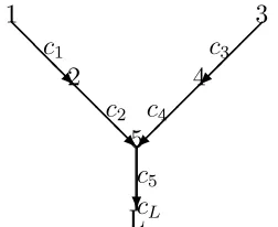
EXAMPLE 1.
1
c1
2
c2
5
3
c3
4
c4
c5
[image:10.595.272.398.285.388.2]LcL
Figure 1
In this example, we have the following P.
P(1) =∅, P(2) ={1}, P(3) =∅, P(4) ={3}, P(5) ={2,4}, P(L) = {5}.
The upstream-downstream structure, denoted as ˆP, is the transitive clo-sure of P. It is defined as a mapping from N ∪ {L} to 2N∪{L} such that for
all i ∈ N ∪ {L} we have j ∈ Pˆ(i) if and only if there exists h1, ..., hm in
N ∪ {L} such that h1 =i, hk+1 ∈ P(hk) for all 1 ≤k ≤m−1, and hm =j. The agents in ˆP(i) are called the upstream agents of i inG.
Given ˆP, its inverse mapping ˆP−1is defined by ˆP−1(i)≡ {j ∈ N∪{L}|i∈
ˆ
P(j)}. We call the agents in ˆP−1(i) the downstream agents of i in G. For
everyS ⊆N, denote ˆP(S) =∪i∈SPˆ(i).
EXAMPLE 1 continued: It is easy to check that
ˆ
P(1) =∅,Pˆ(2) ={1},Pˆ(3) =∅,Pˆ(4) ={3},
ˆ
P(5) ={1,2,3,4},Pˆ(L) ={1,2,3,4,5}.
ˆ
P−1(1) ={2,5, L},Pˆ−1(2) ={5, L},Pˆ−1(3) ={4,5, L},
ˆ
P−1(4) ={5, L},Pˆ−1(5) ={L},Pˆ−1(L) =∅.
Given a network G or ˆP, for any coalition of agents, S ⊆ N ∪ {L}, we can define three different coalitions of agents that are related to S. The
stand-alone counterpart of S is S itself. The Upstream-oriented counterpart of S is the coalition
σ(S)≡S∪Pˆ−1(S), (1) while the Downstream-oriented counterpart of S is the coalition
α(S)≡S∪Pˆ(S). (2)
According to the upstream-downstream structure ˆP, we can define the following three different cost sharing methods for the problem. First, we be-gin with a method which can be considered as being based on the Absolute Territorial Sovereignty (ATS) theory. It is the following so-called Local Re-sponsibility Sharing Method (LRS).
Definition 1 For any C ∈ Rn+1
+ , The Local Responsibility Sharing method
is given by
xLRSi (C) =ci, i= 1, ..., n, L. (3)
Apparently, the LRS method does not depend on ˆP. But, the following two methods depend on ˆP.
Definition 2 The Upstream Equal Sharing method (UES) is defined by
xU ES i (C) =
j∈σ({i})
cj
|α({j})|, i= 1, ..., n, L, (4)
In the UES, an agent’s cost share is the sum of her cost plus the equal sharing of all her downstream costs. This is the so-called Downstream Re-sponsibility, derived from the Unlimited Territorial Integrity theory. Roughly speaking, downstream agents have the rights on thequality of the water they receive. If upstream agents pollute, thus alter the nature of the water flow, upstream agents should be held responsible. In other words, upstream agents have downstream responsibility in sharing their costs. Note that each indi-vidual agent’s responsibility is dependent on ˆP.
In contrast, if we require that all the downstream agents are equally responsible for their upstream costs (the Upstream Responsibility principle), we then have the following Downstream Equal Sharing method (DES).
Definition 3 The Downstream Equal Sharing method is defined by
xDESi (C) =
j∈α({i})
cj
|σ({j})|, i= 1, ..., n, L. (5)
In the DES, an agent’s cost share is the sum of her cost plus the equal sharing of all her upstream costs. This so-called Upstream Responsibility is also derived from the Unlimited Territorial Integrity theory. To see how, think of the dual problem of the polluted river problem, the water sharing problem. In water sharing, downstream agents have the rights on thequantity
of water they can possibly receive from the upstream under the condition that all the upstream agents have received their maximum welfare levels they can possibly achieve given the water resources they control.16 As we mentioned
in the introduction, in Ambec and Sprumont (2002) this argument gives rise to a water sharing method17called the Downstream Incremental Distribution
method, which favors the downstream agents. We argue that when it comes to cost sharing (responsibility), the downstream agents should inherit certain proportion of responsibility in sharing the upstream costs. Like the UES, each individual agent’s specific responsibility also depends on ˆP. But unlike the UES, the DES is based on the Upstream Responsibility principle.
16
This does not mean that upstream agents would use up all the water they control. In fact, they might do better by transferring some water to their downstream counterparts and receiving certain monetary transfers from them. See Ambec and Sprumont (2002).
17
Interestingly, the above three methods coincide with the Shapley values of three different games that can be defined for the problem. These games embody different interpretations of the ATS and the UTI theories.
Specifically, for any given problem (N∪{L}, G, C) we define the following three games: the stand-alone game, the Upstream-oriented game and the
Downstream-oriented game, respectively.
Definition 4 Let(N∪{L}, G, C)be a problem. Define the stand-alone game
Ls.a.(C) as follows:
Ls.a.(C)(∅) = 0, Ls.a.(C)(S) =C(S), S ⊆N ∪ {L}, (6)
where C(S) =
i∈Sci is the total cost of the links associated with S.
Definition 5 Let(N∪{L}, G, C)be a problem. Define the Upstream-oriented game LU(C) as follows:
LU(C)(∅) = 0, LU(C)(S) =C(σ(S)), S ⊆N ∪ {L}. (7)
where σ(S) is defined in (1)
Definition 6 Let (N ∪ {L}, G, C) be a problem. Define the Downstream-oriented game LD(C) as follows:
LD(C)(∅) = 0, LD(C)(S) =C(α(S)), S⊆N ∪ {L}. (8)
where α(S) is defined in (2)
EXAMPLE2. The Upstream-oriented game and the Downstream-oriented game generated from the problem in EXAMPLE 1 are given below. Note that not all coalitional values are listed.
The Upstream-oriented GameLU(C):
LU(C)(1) =c1+c2+c5+cL, LU(C)(3) =c3+c4+c5+cL,
LU(C)(1,2) =c
1+c2+c5+cL, LU(C)(1,3) =c1+c2+c3+c4+c5+cL,
LU(C)(1,2,3) =c
1+c2+c3+c4+c5+cL, LU(C)(1,2,5) =c1+c2+c5+cL,
LU(C)(1,2,3,4) =c
1+c2+c3+c4+c5+cL, LU(C)(1,3,4,5) =c1+c2+c3+c4+c5+cL,
LU(C)(1,2,3,4,5) =c
1+c2+c3+c4+c5+cL, LU(C)(1,2,3,4,5, L) =c1+c2+c3+c4+c5+cL. The Downstream-oriented GameLD(C):
LD(C)(1) =c
1, LD(C)(3) =c3, LD(C)(5) =c1+c2+c3+c4+c5,
LD(C)(L) =c1+c2+c3+c4+c5+cL, LD(C)(1,2) =c1+c2, LD(C)(1,3) = c1+c3,
LD(C)(1,5) =c1+c2+c3+c4+c5, LD(C)(1, L) =c1+c2+c3+c4+c5+cL,
LD(C)(1,2,3) = c
1+c2+c3, LD(C)(2,5, L) =c1+c2+c3+c4+c5+cL,
LD(C)(1,2,3,4) =c1+c2+c3+c4, LD(C)(1,3,4,5, L) =c1+c2+c3+c4+c5+cL,
LD(C)(1,2,3,4,5) = c
1+c2+c3+c4+c5, LD(C)(1,2,3,4,5, L) =c1+c2+c3+c4+c5+cL. In the cooperative game theory, the Shapley value (Shapley, 1953) is the
most important solution concept. It is given below.
Definition 7 For any game C : 2N →R, the Shapley value is given by
xShi (C) =
S∋i
(n− |S|)!(|S| −1)!
n! (C(S)−C(S\ {i}), i= 1, ..., n. (9)
The Shapley value of an agent can be regarded as an average of the marginal cost incurred by the agent to each and every coalition of other agents.
Another important solution concept is the core. In the context of cost sharing, a core allocation is an allocation which cannot be dominated by an alternative allocation in which some agent or coalition of agents can have their cost shares reduced by themselves and be better off given their stand-alone cost. In other words, once a core allocation is proposed, no coalition of agents has the incentive to change the allocation. The core of a game is the set of all core allocations. In general, a game may have an empty core.
core. A (cost) game is concave if an agent’s marginal cost is non-increasing as the agent joins larger coalitions. Formally, a game C(·) is concave if
C(S∪i)−C(S)≥C(T ∪i)−C(T),∀S ⊆T ⊆N, i /∈T.
In the next section, we will show that the three games defined above are all concave. Thus, their Shapley values are in the core of the corresponding games. Moreover, we will show that the three methods coincide with the Shapley values of the three games, respectively. Therefore, the solutions by the three methods are all core allocations of the corresponding games.
We conclude this section by pointing out that while the LRS and the UES are the extensions of the two corresponding methods in Ni and Wang (2007), the DES is closely related to the well-known airport landing fee solution (Littlechild and Owen, 1973, 1977).18 This can be shown by considering the
following special case where the tree network is a line-tree.
1 c12 c23 c34 c4L, cL
The Upstream Equal Sharing is the following:
xU ES
1 (C) = c1+
1 2c2+
1 3c3+
1 4c4+
1 5cL,
xU ES
2 (C) =
1 2c2+
1 3c3+
1 4c4+
1 5cL,
xU ES
3 (C) =
1 3c3+
1 4c4+
1 5cL,
xU ES
4 (C) =
1 4c4+
1 5cL,
xU ES
L (C) = 1 5cL,
and it coincides with the UES in Ni and Wang (2007).
18
The Downstream Equal Sharing, on the other hand, coincides with the airport landing fee solution.
xDES
1 (C) =
1 5c1
xDES
2 (C) =
1 5c1+
1 4c2
xDES
3 (C) =
1 5c1+
1 4c2+
1 3c3
xDES
4 (C) =
1 5c1+
1 4c2+
1 3c3+
1 2c4
xDES
L (C) = 1 5c1+
1 4c2+
1 3c3+
1
2c4+cL
3
Characterizations of the LRS, the UES and
the DES Methods
3.1
A Characterization of the LRS Method
In order to characterize the LRS method, similar to Ni and Wang (2007), we need the following axioms.
Additivity: For anyC1 = (c1
1, . . . , c1n, c1L)∈Rn++1andC2 = (c21, . . . , c2n, c2L)∈
Rn+1
+ , we have xj(C1+C2) =xj(C1) +xj(C2) for all j ∈N ∪ {L}.
Additivity is a classical axiom in the cooperative game theory (Shap-ley, 1953) and the cost sharing literature (Moulin, 2002). As a mathemati-cal structural invariance axiom, Additivity itself has no normative content. However, for our pollution cost sharing problem, we can provide the follow-ing interpretation.
No Blind Costs: For any i ∈ N ∪ {L} and any C ∈Rn+1
+ , if ci = 0, then
xi(C) = 0.
No Blind Costs says that if an agent’s cost is zero, then the agent’s cost share should be zero as well. This axiom rules out cross subsidization be-tween the agents. If an agent’s cost is zero, it means that there is no pollution (cost) at the agent’s location. Therefore, the agent neither pollutes herself and her downstream nor is polluted by her upstream agents. Thus, the agent shouldn’t bear any cost.
Efficiency: n+1
j=1 xj =nj=1+1cj.
Efficiency is always satisfied by a cost sharing method by definition. Nev-ertheless, we mention it explicitly in all our characterizations as it is the only axiom that is related to economic efficiency.19
Theorem 1 The Local Responsibility Sharing method is the unique method that satisfies Additivity, No Blind Costs and Efficiency. It coincides with the Shapley value of the stand-alone game of the problem. Moreover, it is in the core of the game.
The proof of theorem is similar to the proofs of Theorem 1, Propositions 1 and 2 in Ni and Wang (2007). We omit it.
3.2
A Characterization of the UES Method
In this subsection, we provide a characterization of the Upstream Equal Sharing method and show that it coincides with the Shapley value of the Upstream-oriented game generated from the problem. Moreover, it is in the core.
19
Recall that for a given cost functionC = (c1, c2, . . . , cn, cL), the associated Upstream-oriented game is defined by
LU(C)(S) =C(σ(S)) =
j∈σ(S)
cj, S ⊆N ∪ {L},
where σ(S) =S∪Pˆ−1(S) =S∪(
j∈SPˆ−1(i)). Note that
LU(C)(N ∪ {L}) =C(σ(N ∪ {L})) = C(N ∪ {L}).
The Upstream Equal Sharing method is repeated below.
xU ES i (C) =
j∈σ({i})
cj
|α({j})|, i= 1, ..., n, L, (10)
where |α({j})| is the number of the elements in α({j}), and α({j}) =
{j} ∪Pˆ({j}) ={j} ∪Pˆ(j).
We introduce the following axioms.
Independence of Upstream Costs: For any i ∈ N ∪ {L}, any C, C′ ∈
Rn+1
+ such thatcl =c′l, l∈Pˆ−1(i), we havexj(C) =xj(C′) for allj ∈Pˆ−1(i). This axiom is based on the Downstream Responsibility principle, which is a responsibility version of the theory of the Unlimited Territorial Integrity as we discussed in the introduction. It says that an agent’s cost share only depends on her own pollution cost as well as all her downstream costs, but not on upstream costs for which she is assumed not responsible.
Upstream Symmetry: For any i ∈ N ∪ {L}, for all j, k ∈ α({i}) =
{i} ∪Pˆ(i), we have
xj(0, ...,0, ci,0, ...,0) =xk(0, ...,0, ci,0, ...,0).
is hard to tell exactly how much each upstream agent contributes to the given downstream cost. Moreover, the axiom implies that any agent, no matter how far she is from any of her downstream agents, her responsibility remains the same.
The following Independence of Irrelevant Costs axiom is essential in all our characterizations in this paper. As we discussed before, it imposes an upper bound on an agent’s responsibility, i.e., an agent is not responsible for any cost that is irrelevant to her. Formally,
Independence of Irrelevant Costs: For any i ∈ N ∪ {L}, for all j ∈ N ∪ {L} \( ˆP(i)∪ {i} ∪Pˆ−1(i)), we have
xj(0, ...,0, ci,0, ...,0) = 0.
This is a compelling axiom since if two agents are not related to each other in the river network in terms of the upstream-downstream relationship, each agent wouldn’t affect the other in pollution cost sharing. Thus, it is plausible to require that neither agent should be responsible for the cost of the other. This axiom allows us to extend the responsibility theory derived from the theory of the Unlimited Territorial Integrity to a tree network.
Note that in Ni and Wang (2007), each agent is either an upstream or a downstream of all other agents in the linear river model. But in our tree model, the upstream-downstream relation on the agents is a partial order.
Now we are ready to state the following theorem.
Theorem 2 The Upstream Equal Sharing method is the unique method that satisfies Additivity, Independence of Upstream Costs, Upstream Symmetry, Independence of Irrelevant Costs and Efficiency. Moreover, it coincides with the Shapley value of the Upstream-oriented game of the problem, and it is in the core of the game.
Proof: We divide the proof into three steps.
Step 1. First, we show that the Shapley value xSh of the Upstream-oriented game LU(C) coincides with the UES method xU ES.
By the definition of the Upstream-oriented game, for any
where 1 is the kth component of then+ 1-dimensional vectorCk, the corre-sponding Upstream-oriented game is given by
LU(Ck)(S) = 0 if S ⊂N ∪ {L}\α({k}) andLU(Ck)(S) = 1 otherwise. Clearly, all agents inN∪{L}\α({k}) are dummy agents and all agents in
α({k}) are symmetric. Thus the Shapley value of the game LU(Ck) is given by
xSh i (L
U(Ck)) =
1
|α({k})|, i∈α({k})
0, otherwise (11) for all i∈N ∪ {L}.
Since the cost vectors, Ck(k ∈ {1, . . . , n, L}), form a basis of Rn+1, for
any C ∈ Rn+1
+ , it can be uniquely written as C =
k∈N∪{L}ck·Ck. By the definition of the Upstream-oriented game, for ∅ =S ⊆N ∪ {L}, we have
LU(C)(S) =
j∈σ(S)
cj
=
j∈σ(S)
(
k∈N∪{L}
[ck·Ck]j)
=
k∈N∪{L}
ck·(
j∈σ(S)
[Ck] j)
=
k∈N∪{L}
ck·LU(Ck)(S)
where [C]j is thejth component of the vectorC. Because the Shapley value satisfies Additivity, we have
xShi (L U
(C)) =
k∈N∪{L}
ck·xShi (L U
(Ck))
=
k∈N∪{L}\σ({i})
0 +
k∈σ({i})
ck
|α({k})|
= xU ESi (C) for all i∈N ∪ {L}.
We first show thatxU ES satisfies these five axioms. Additivity is straight-forward. To show that xU ES satisfies Independence of Upstream costs, for any i∈N ∪ {L}, any C, C′ ∈Rn+1
+ such that cl =c′l, l∈Pˆ−1(i), then for all
j ∈Pˆ−1(i), we have
xU ES
j (C) =
l∈σ({j})
cl
|α({l})|
=
l∈{j}∪Pˆ−1(j)
cl
|α({l})|
=
l∈{j}∪Pˆ−1(j)
c′
l
|α({l})|
= xU ESj (C′)
since j ∈Pˆ−1(i)⇒Pˆ−1(j)⊆Pˆ−1(i).
To see that xU ES satisfies Upstream Symmetry, for anyi∈N ∪ {L}, for allj, k ∈α({i}) ={i} ∪Pˆ(i), we have
xU ESj (0, ...,0, ci,0, ...,0) =
l∈σ({j})
cl
|α({l})|
=
l∈{j}∪Pˆ−1(j)
cl
|α({l})|
= ci
|α(i)|
=
l∈{k}∪Pˆ−1(k)
cl
|α({l})|
=
l∈σ({k})
cl
|α({l})|
= xU ESk (0, ...,0, ci,0, ...,0).
We now show thatxU ES satisfies Independence of Irrelevant Costs. Since
j ∈N∪{L}\( ˆP(i)∪{i}∪Pˆ−1(i)), we havei /∈Pˆ−1(j). Otherwise,i∈Pˆ−1(j)
implies j ∈ Pˆ(i), a contradiction. Thus, if C = (0, ...,0, ci,0, ...,0), then
cl= 0 for all l∈ {j} ∪Pˆ−1(j) =σ(j). We therefore have
xU ESj (C) =
l∈σ({j})
cl
Finally, in Step 1 we have shown that xU ES is the Shapley value of the Upstream-oriented game. Since the Shapley value satisfies Efficiency, xU ES also satisfies Efficiency.
Now we show that the UES is the only method satisfying the five ax-ioms. Suppose that a cost sharing method x satisfies the five axioms. Fix a arbitrary tree consisting of n+ 1 nodes. For any k ∈ {1,2, . . . , n, L}, let
Ck = (0,0, . . . ,0,1,0, . . . ,0) where 1 is the kth component of the n + 1-dimensional vector Ck. By Independence of Upstream Costs, x
j(Ck) = 0 for all j ∈ Pˆ−1(k). By Independence of Irrelevant Costs, x
j(Ck) = 0 for all
j ∈N ∪ {L}\( ˆP(k)∪σ({k})). By Upstream Symmetry, xj(Ck) =xj′(Ck) =
β ≥0 for all j, j′ ∈α({k}). By Efficiency, we have
j∈N∪{L}
xj(Ck)
=
j∈Pˆ−1(k)
xj(Ck) +
j∈{k}∪Pˆ(k)
xj(Ck) +
j∈N∪{L}\( ˆP(k)∪{k}∪Pˆ−1(k))
xj(Ck)
= 0 +
j∈α({k})
β+ 0
= β× |α({k})|
= 1
therefore xj(Ck) = |α({1k})| if j ∈α({k}) and xj(Ck) = 0 otherwise. Again, for anyC ∈Rn+1
+ , it can be uniquely written asC = (c1, . . . , cn, cL) =
k∈N∪{L}ck·Ck. By Additivity, we have
xi(C) = xi(
k∈N∪{L}
ck·Ck)
=
k∈N∪{L}
ck·xi(Ck)
=
k∈N∪{L}\( ˆP(i)∪σ({i}))
0 +
k∈Pˆ(i)
0 +
k∈σ({i})
ck
|α({k})|
= xU ES i (C) for all i∈N ∪ {L}.
i∈N ∪ {L}, all S, T ⊂(N ∪ {L})\{i}and S ⊂T, we have
LU(C)(S∪ {i})−LU(C)(S)≥LU(C)(T ∪ {i})−LU(C)(T). (12)
Suppose that S ⊂ T and i /∈ T. Let HU
S = σ(S∪ {i})\σ(S) and HTU =
σ(T ∪ {i})\σ(T). We claim that HU
T ⊆HSU. Since
HU
S = σ(S∪ {i})\σ(S)
= S∪ {i} ∪Pˆ−1(S)∪Pˆ−1(i)\(S∪Pˆ−1(S)) = {i} ∪Pˆ−1(i)\(S∪Pˆ−1(S)),
and
HTU ={i} ∪Pˆ−1(i)\(T ∪Pˆ−1(T)),
and that
T ∪Pˆ−1(T)⊇S∪Pˆ−1(S),
we thus have
HU T ⊆H
U S. Therefore,
LU(C)(S∪ {i})−LU(C)(S) =
j∈σ(S∪i)
cj−
j∈σ(S)
cj
=
j∈HU S
cj
≥
j∈HU T
cj
=
j∈σ(T∪i)
cj −
j∈σ(T)
cj
= LU(C)(T ∪ {i})−LU(C)(T).
3.3
A Characterization of the DES Method
We now provide a characterization of the Downstream Equal Sharing method and show that it coincides with the Shapley value of the Downstream-oriented game of the problem and, moreover, is in the core of the game.
Recall that for a given cost functionC = (c1, c2, . . . , cn, cL), the Downstream-oriented game is defined by
LD(C)(S) = C(α(S)) =
j∈α(S)
cj, S ⊆N ∪ {L},
where α(S) =S∪Pˆ(S) =S∪(
j∈SPˆ(i)). Note that
LD(C)(N ∪ {L}) =C(α(N ∪ {L})) =C(N ∪ {L}). The Downstream Equal Sharing method is repeated below.
xDESi (C) =
j∈α({i})
cj
|σ({j})|, i= 1, ..., n, L, (13)
where σ({j}) ={j} ∪Pˆ−1({j}) ={j} ∪Pˆ−1(j).
To characterize the DES, we need the following two axioms.
Independence of Downstream Costs: For any i∈N∪ {L}, anyC, C′ ∈
Rn+1
+ such that cl =c′l, l∈Pˆ(i), we have xj(C) =xj(C′) for all j ∈Pˆ(i). The Independence of Downstream Costs imposes an upper bound on an agent’s cost share, i.e., it wouldn’t be dependent on her downstream agents’ costs. This axiom, as we discussed in the introduction on the Downstream Responsibility principle, says that an agent’s responsibility in cost sharing is directed toward her upstream rather than the downstream. This alternative theory is in contrast to the Upstream Responsibility. Note that this version of the responsibility theory is aderivedresponsibility from the dual problem, namely the water sharing problem (Ambec and Sprumont, 2002).
Downstream Symmetry: For any i ∈ N ∪ {L}, for all j, k ∈ σ({i}) =
{i} ∪Pˆ−1(i), we have
Similar to the Upstream Symmetry, the Downstream Symmetry treats all downstream agents equally in terms of responsibility for a given upstream cost. Again this axiom ignores the physical distance between the agents. In other words, all agents, no matter how far they are from any of their given upstream agents, are equally responsible for their costs. This axiom together with the previous axiom, specifies the downstream responsibility.
Now we state the following theorem.
Theorem 3 The Downstream Equal Sharing method is the unique method that satisfies Additivity, Independence of Downstream Costs, Downstream Symmetry, Independence of Irrelevant Costs and Efficiency. Moreover, it coincides with the Shapley value of the Downstream-oriented game of the problem and, is in the core of the game.
Proof: The proof is analogous to the proof of Theorem 2. To do that, we only need to replace the Independence of Upstream Costs and the Upstream Symmetry in the proof of Theorem 2 by the Independence of Downstream Costs and the Downstream Symmetry, respectively. It is also straightforward to check that the Downstream Equal Sharing method coincides with the Shapley value of the Downstream-oriented game of the problem and is in the core of the game. We omit the details.
The UES and DES methods provide the upper and lower bounds for an agent’s cost shares. Apparently, the upstream agents prefer the DES but the downstream agents prefer the UES. Some compromise between the two solutions should be made. For example, in realistic situations, a weight can be assigned to each agent according to the agent’s observable characteristics such as the agent’s pollutant emission/abatement level, willingness-to-pay or ability-to-accept, the size of the agent (e.g., population), the distance between the agent to the Lake, etc. Costs can be then allocated according to a weighted average rather than the equal division of the costs among the relevant agents.
3.4
An Example: the Baiyangdian Lake Catchment
suggested by our model bring forward two extreme viewpoints between which policy makers can balance their choices in allocating the total costs of the project.
The Baiyangdian Lake, the largest remaining semi-closed freshwater body in the northern China, is one of the most important and vulnerable ecosys-tems. It lies in the middle reaches of Daqing River Basin and ultimately discharges in Bohai Gulf and the Yellow Sea. All of the lake body is located in Anxin and Xiong counties of Baoding Municipality. The lake has a surface area of 366 km2 and consists of a series of natural low-lying depressions and
reed marshes. There are four large-scale reservoirs upstream of the lake, in-cluding Angezhuang, Longmen, Wangkuai, and Xidayang with water flowing into the lake via eight rivers.
Historically, the lake served many environmental and economic purposes and was called as the “kidney” of the northern China. Its strategic position is reflected by its major role in regulating floodwater discharges and water levels, and subsequently moderates waterlogging. The lake has been an eco-nomically important source of freshwater fish and reed production as well as a source for drinking water and irrigation.
However, over the last four decades, the size of the lake has decreased by almost half because of controlled water flows, and soil erosion, rising population, expanded agricultural and industrial activities, limited solid and wastewater disposal measures in the upstream and within the lake area.20
The lake has been a major depository of wastewater discharges, pollutant substances, and sediments. Almost all the subproject urban areas discharge untreated wastewater into the adjacent rivers and eventually to the lake. Major industries within the service areas include tanneries, textile, paper, automobile, fertilizer, chemicals, and machinery plants which are all polluting industries. It is estimated that half of the pollution originates from the upstream, while the other half emanates from the population of more than 200,000 living in the lake’s wetlands and surrounding areas.
20
Figure 2. Wastewater treatment plants in Baiyangdian area
Eutrophication of the lake has become a serious problem. Water quality deteriorated from class III to classes IV and V over the past four decades.21
In 2008, an integrated Project cofinanced by the Asian Development Bank (ADB) and Global Environment Facility (GEF), with a total investment of US$203.7 million, helps to construct 13 wastewater treatment plants in the upstream of Lake Baiyangdian, along with other facilities such as water sup-ply, reforestation, rehabilitation of watershed, flood control etc. The Project reduces the COD by 36,850 tons/year (or 365,000 m3/day of wastewater)
21
upon completion. It also reduces morbidity rates by 10% and improves sani-tation and hygiene for 1.12 million people and maintains a sustainable healthy water level of the lake. The locations of the wastewater treatment plants are shown in Figure 2.
The 13 wastewater treatment plants located in the main counties and townships in the upstream are essential for pollution reduction in Lake Baiyang-dian. Other subprojects around the lake such as reforestation and wastershed rehibilitation also contribute to the restoration of the lake’s environmental and economic functions. The investment figures for the subprojects are round up and depicted in Figure 3 with an illustration of the tree-structure water flows. The unit is million US$.22
LakeBaiyangdian $56
Player2: Xinxing
$8
Player3:Liushi
$7 Player1:Li
$9
Player12:Dingxing
$11
Player5:Dingzhou
$5
Player6:Mancheng
$6 Player7:Xushui
$7
Player9:Xiong
$9
Player10:Wenquancheng
$7 Player8:Anxin
$3
Player13:Baigou
$8 Player11:Yi
$8 Player4:Tang
[image:28.595.126.476.330.538.2]$4
Figure 3. Illustration of the Baiyangdian Lake Project
According to the formulae developed in this paper, we calculate the two cost sharing solutions based on the UES and DES methods, respectively.
22
First, we calculate the UES sharing:
xU ES
1 (C) =c1+13c3+141cL = 463 , xU ES2 (C) =c2+13c3+ 141cL= 433,
xU ES
3 (C) = 13c3+ 1 14cL=
19
3, x
U ES
4 (C) =c4+c25 +10c8 +c14L = 16810,
xU ES
5 (C) = 12c5+ 1 10c8+
1 14cL=
108 10, x
U ES
6 (C) =c6+101 c8 +141cL= 13310,
xU ES
7 (C) =c7+101 c8+ 141cL= 13310, xU ES8 (C) = 101 c8+ 1
14cL= 4310,
xU ES
9 (C) =c9+c510 + c108 +c14L = 11210, xU ES10 (C) = 15c10+ 1 10c8+
1 14cL =
62 10,
xU ES
11 (C) =c11+ 13c13+15c10+ 101c8+141 cL = 20315,
xU ES
12 (C) =c12+ 13c13+15c10+ 101c8+141 cL = 29815,
xU ES
13 (C) = 13c13+ 1 5c10+
1 10c8+
1 14cL=
133 15,
xU ES
L (C) = 141cL= 4.
Then, we calculate the DES sharing:
xDES
1 (C) = 13c1 = 3, x
DES
2 (C) = 13c2 = 8 3,
xDES
3 (C) = 13c1+ 1 3c2+
1 2c3 =
55
6, x
DES
4 (C) = 14c4 = 3 2,
xDES
5 (C) = 13c5+ 1 4c4 =
35
6, x
DES
6 (C) = 13c6 = 3,
xDES
7 (C) = 13c7 = 3,
xDES
8 (C) = c28 +
c5+c6+c7+c10
3 +
c4+c9+c13
4 +
c11+c12
5 =
1363 60 ,
xDES
9 (C) = 14c9 = 5 4,
xDES
10 (C) = 15c10+ 1
5(c11+c12) + 1
4 (c9+c13) = 563
60,
xDES
11 (C) = 15c11= 8
5, x
DES
12 (C) = 15c12 = 11
5 ,
xDES
13 (C) = 15(c11+c12) + 1 4c13 =
29 5,
xDES
L (C) = c3+2c8 +
c1+c2+c5+c6+c7+c10
3 +
c4+c9+c13
4 +
c11+c12
5 +cL= 87 53 60.
4
Concluding Remarks
We studied the cost sharing problem in a polluted river network. We pro-posed three cost sharing methods for the problem and provided their ax-iomatic characterizations. Our characterizations are based on the two well-known theories in international disputes. We also showed that these three methods are the Shapley values of the three associated games of the problem. Moreover, they are in the cores of the three games, respectively.
Our paper can be extended in a number of directions. For example, between the two opposing versions of responsibility (the UR and the DR), a range of them can be proposed. Accordingly, a set of methods can be generated by considering all the weighted averages of the UES and the DES methods. We can make the weights depending on the weights we assign to each and every agent. In assigning weights to the agents, we can take into account the differences between the agents in, e.g., population, pollutant emission, the location of the agent in the network, etc.
A more challenging but perhaps more useful extension of our work could be to combine the water sharing problem with the water pollution cost shar-ing problem. In fact, Weber (2001) has considered the problem of allocatshar-ing water and pollution rights along a river. But, in Weber (2001), there is a single source of water. There are no branches or inflows at various locations of the agents. Also the pollution rights are exogenously assigned by a regu-lator. Agents engage in trading water rights and pollution rights by playing a noncooperative game. Our approach in this paper is axiomatic and can be considered as the reverse of the Weber’s. We begin with ceratin normative principles (axioms). The cost sharing methods determined by the various combinations of the axioms would, in effect, determine or imply implicitly an assignment of property rights.
References
[1] Aadland D. and Kolpin V., 1998. Shared irrigation costs: An empirical and axiomatic analysis. Mathematical Social Sciences 849, 203-218.
[3] Ambec, S., Ehlers, L., 2008a. Sharing a river among satiable agents.
Games and Economic Behavior, 64(1): 35-50
[4] Ambec, S., Ehlers, L., 2008b. Cooperation and equity in the river sharing problem. In Game Theory and Policy Making in Natural Resources and the Environment, edited by Arial Dinar et al., Routledge Publishers.
[5] Ambec, S., Sprumont, Y., 2002. Sharing a River. Journal of Economic Theory 107, 453-462.
[6] Ansink, E. and Ruijs, A., 2008, Climate change and the stability of water allocation agreements, Environmental and Resource Economics, 41:249-266
[7] Barrett, S., 1994. Conflict and cooperation in managing international water resources, Working Paper 1303, World Bank, Washington.
[8] Coase, R., 1960. The problem of social cost. Journal of Law and Eco-nomics 1, 1-14.
[9] Godana, B., 1985. Africa’s shared water resources, France Printer, Lon-don.
[10] Hung, M-F. and Shaw, D., 2005, A trading-ratio system for trading water pollution discharge permits,Journal of Environmental Economics and Management, 49:83-102
[11] Kilgour, M. and Dinar, A., 1996. Are stable agreements for sharing international river waters now possible? Working Paper 1474, World Bank, Washington.
[12] Kilgour, M. and Dinar, A., 2001, Flexible water sharing within an inter-national river basin, Environmental and Resource Economics, 18:43-60
[13] Littlechild, S. and Owen, G., 1973. A Simple Expression for the Shapley Value in a Special Case. Management Science 20, 370-372.
[15] Marchiori, C., 2010, Concern for fairness and incentives in water nego-tiations,Environmental and Resource Economics 45:553-571
[16] Moulin, H., 2002. Axiomatic cost and surplus sharing. In: Arrow, K.J., Sen, A.K., and Suzumura, K. (Eds.), Handbook of Social Choice and Welfare, Volume 1, North-Holland, Amsterdam.
[17] Moulin, H., 2011. Cost sharing in networks: some open questions. Work-ing paper, Rice University.
[18] Ni, D. and Wang, Y., 2007. Sharing a Polluted River. Games and Eco-nomic Behavior 60, 176-186.
[19] Van den Brink, J. R. and Gilles, R. P., 1996. Axiomatizations of the Conjunctive Permission Value for Games with Permission Structures.
Games and Economic Behavior 12, 113-126.
[20] Shapley, L. S., 1953. A Value for n-Person Games. In: H. W. Kuhn and A. W. Tucker (Eds.), Contributions to the Theory of Games II, Annals of Mathematics Studies 28, 307-17.
[21] Shapley, L. S. 1971. Core of convex games. International Journal of Game Theory 1: 11-26
[22] Wang, Y.. 2011. Trading water along a river. Mathematical Social Sci-ences 61: 124-130