Income Transfer as Model of Economic Growth

Munich Personal RePEc Archive

Income Transfer as Model of Economic

Growth

Costa Junior, Celso Jose and Sampaio, Armando Vaz and

Gonçalves, Flávio de Oliveria

Universidade Positivo - UP, Universidade Federal do Paraná - UFPR

10 December 2012

Online at

https://mpra.ub.uni-muenchen.de/45494/

Income Transfer as Model of Economic

Growth

Celso Jose Costa Junior

Armando Vaz Sampaio

Flavio de Oliveira Goncalves

First Draft Version

Abstract

This work aims to study the main Brazilian economic growth influenced by an income transfer program. For this purpose, we used the DSGE ap-proach. The estimation of the parameters was performed using the Bayesian methodology and analysis of results was done by impulse response func-tions. The basic characteristic of this paper is to use two types of consumers: ricardian individuals and non-ricardian individuals. The first agents maxi-mize intertemporally its utility function, while the second type of agents is limited to consume the amount received through income transfer. The results show that implantation this program brings positive returns for the whole economy, except for individuals ricardian.

Keyword: DSGE Models; Bayesian Estimation; and Income Transfers.

JEL: C63; E37; E62.

∗_{Professor of Business School - Universidade Positivo}

1

Introduction

This study aims to examine the proposal of economic growth adopted by the Brazilian government in recent years - consumption fostered by income trans-fer policy. Considering that in December 2009, the Bolsa Familia1 represented 12,370,915 benefits, and since the consolidation of this program, it settled a broad debate about its potential to reduce poverty and promote fall in income inequality existing in Brazil (Castro and Modesto , 2010).

The per capita income in Brazil increased 1.4% and 1% per year in the periods 1981-1995 and 1995-2003, respectively. After 2003 the combination of renewed economic growth with the expansion of income transfer programs promoted, sig-nificantly, the improve of per capita income, 5% per year (Castro and Modesto , 2010). Note that the per capita income grew 3.5 times over the period of expan-sion of these programs when compared to the other two periods. The modeling tool DSGE (Dynamic Stochastic General Equilibrium) was chosen due its ability to analyze the movements of economic variables in relation to an exogenous shock (Income Transfer). Through this approach, it is expected to study the behavior of key macroeconomic variables after the implementation of the social program.

Over the past twenty years have seen tremendous advances in tools math-ematical, statistical, probabilistic and computing available for applied macroe-conomists. This huge set of tools has changed the way researchers approach test models, validate theories or simply seek regularities in the data. The rational ex-pectations and the calibration revolutions also forced researchers to try to build a stronger bridge between theoretical and applied work, a bridge was absent in most applied exercises conducted in the 1970s and 1980s (Canova , 2007). The work of Kydland and Prescott (1982)”Time to Build and Aggregate Fluctuations” rev-olutionized modern macroeconomics, but the first steps of this methodology are given by Ramsey [(Ramsey , 1927) and (Ramsey , 1928)], Cass (1965), Koop-mans (1965) and Brock and Mirnam (1972).

One key assumption of DSGE models is that individuals are optimizers and, therefore, they can determine an optimal basket of consumption since one can to be separate to his income, fulfilling the hypothesis of the life cycle permanent

1_{The Bolsa Familia Program was created in 2003 with the goal of unifying the income}

income. For this, individuals use the variable investment to carry income intertem-porally. However, empirical evidence shows that there is a certain relationship be-tween consumption and current income [(Campbell and Mankiw , 1989), (Deaton , 1992), (Wolff , 2003), and (Johnson et al , 2006)], demonstrating a breach of that basic assumption.

The economic literature shows different elements that cause deviations from the theory of the life cycle permanent income. The main explanation for this result is due to the capital market is not perfect and therefore the existence of liquidity constraint for some individuals. Assuming this explanation, this paper develops a model in which there are two types of agents: ricardian agents and agents which have liquidity constraint denominated as non-ricardian (rule-of-thumb). In prac-tice, many agents are subject to liquidity constraint but would like to raise the present consumption by future income, but they do not have access to credit. This implies that these agents can not maximize their utility intertemporal and their consumption is restricted to current income.

The calibration approach for parameter values is not the most appropriate, because their values are always conditional on a particular model. So, it is not in-dicated to import values from another model. Due to this, the estimation of DSGE models using methodologies Bayesian became the estimation method most com-monly used among macroeconomists. Thus, we were decided to estimate the structural model using this approach.

The results demonstrate that the introduction of the income transfer program brings positive returns for the whole economy, except for ricardian individuals be-cause consumption and wage level of these agents remains below its steady state throughout the simulation2.

Besides this introductory section, this paper is structured as follows: section two describes the DSGE model; the third section deals with the estimation of the model parameters; section four shows the results; and finally, conclusions are drawn.

2_{The data used in the estimations are given annual GDP growth and aggregate consumption in}

2

Model

This section shows the economic model this work. It is a simple model con-sisting of households and firms (endogenous agents), and the Government as an exogenous agent (represented in the payment of income transfers)3. Moreover, the model is closed and no financial market.

2.1

Households

The first agent of this model is the representative agent households (ricardian and non-ricardian). The ricardian agent maximizes his utility function (which repre-sents his instant happiness) by choosing consumption and leisure, subject to his budget constraint. Already the non-ricardian merely consumes the transfers re-ceived from the Government.

The most common form to represent the consumption of non-ricardian agents is to possible that they may optimize his utility intratemporal using his disposable income (Cj=W−taxes) [(Gali et al , 2007), (Itawa , 2009), (Coenen and Straub, 2004), (Furlanetto and Seneca , 2007), (Dallari , 2012), (Colciago et al , 2006) and (Mayer and Stahler , 2009)], there are other authors who assume that these agents receive wage with government transfers (Cj =W+trans f ers)[(Fornero , 2010), (Swarbrick , 2012), (Forni et al , 2009) and (Monastier , 2012)]. However, this work follows the form shown by Vereda and Cavalcanti (2010), in which the rev-enue non-ricardian agent is limited to a transfer of income from the Government. But unlike these authors, this article works with the stochastic shock occurring in public income transfer to the non-ricardian agents.

2.1.1 Ricardian Consumers

It is assumed that each ricardian agent maximizes his utility choosing intertem-poral consumption,{Ci,t}_t∞₌₀, and leisure,{1−Li,t}∞_t=0. Ricardian agents’

prefer-ences are defined by the following utility function:

3_{The idea of letting the simple model is to keep the focus on key variables this work, C and}

U=Et

∞

∑

t=0

βt[γlogCi,t+ (1−γ)log(1−Li,t)]

where Et is the expectations operator, β is the intertemporal discount rate, γ ∈ (0,1)is the share of consumption in the utility of ricardian individuals.

The budget constraint says that consumption plus investment do not exceed the sum of the revenues coming from labor and capital:

(Ci,t+Ii,t)Pt =WtLi,t+RtKi,t (1)

whereWt is the wage,Rt is the rate of return on capital,Ki,t is the stock of capital, Li,t is the amount of work andPtand is the price level, which is normalized to one.

The process of capital accumulation is defined by:

Ki,t+1= (1−δ)Ki,t+Ii,t (2)

whereδ is the depreciation rate.

Using (2) in (1), we obtain the budget constraint of the agent ricardian:

Ci,t+Ki,t+1=WtLi,t+ (Rt+1−δ)Ki,t (3)

The corresponding Lagrangian problem faced by ricardian consumers is as follows:

max

Ci,t,Li,t,Ki,t

L _=Et

∞

∑

t=0

βt{γlogCi,t+ (1−γ)log(1−Li,t)

−λt[Ci,t+Ki,t+1−WtLi,t−(Rt+1−δ)Ki,t]

Thus, we arrive at the first order conditions of the above problem:

∂L

∂Ci,t

= γ

Ci,t

∂L

∂Li,t

=− (1−γ)

(1−Li,t)+λtWt =0 (5)

∂L

∂Ki,t

=βEtλt[Rt+1−δ]−λt−1=0 (6)

Combining equations (4) and (5), it is obtained the equation of the work sup-ply ricardian consumers:

(1−γ)

γ

Ci,t

(1−Li,t) =Wt (7)

And using equations (4) and (6), we arrive at the Euler equation for consump-tion:

1

Ci,t−1

=βEt 1 Ci,t

(Rt+1−δ) (8)

2.1.2 Non-Ricardian Consumers

Non-ricardian consumers have a behavior simpler. The idea is that these individ-uals do not participate in the labor market getting their consumption limited to government transfers4. Under this hypothesis:

Cj,t =Trt (9)

whereTrt is the income transfer to non-ricardian consumer j.

Payment of income transfer follows a stochastic process AR (1):

4_{Proof of equation (9): If to be in the Bolsa Familia Program is necessary that the family has}

Trt=ρTrt−1+ε (10)

whereεis the error term.

2.1.3 Aggregation

The aggregate consumption of this work follows the most common functional form (Ct =ωCi,t+ (1−ω)Cj,t) found in the main works of this type of literature

[(Bosca et al, 2010), (Gali et al , 2007), (Itawa , 2009), (Coenen and Straub, 2004), (Furlanetto and Seneca , 2007), (Dallari , 2012), (Mayer et al , 2010), (Stahler and Thomas , 2011), (Swarbrick , 2012), (Motta and Tirelli , 2010), (Diaz, 2012), (Colciago , 2011), (Mayer and Stahler , 2009) and (Forni et al , 2009)].

Thus, the aggregate consumption is performed as follows:

Ct=ωCi,t+ (1−ω)Cj,t (11)

whereω the population share of ricardian consumers.

2.2

Firms

The firms’ problem is to choose optimal values for the use of production factors, capital and labor. It is assumed that both markets for goods and services as factor markets are perfectly competitive. Firms acquire capital and work of households in order to maximize its profit, taking as prices given. The production function is given by:

Yt=AtKtαL1−αt (12)

whereAt is the total factor productivity,α is the capital participation in the

The productivity5follows a stochastic process AR (1) described below:

At =ρAt−1+εA (13)

whereεA is the error term.

The problem of the firm is to maximize its profit function:

π=AtKtαL1−αt −WtLt−RtKt (14)

The maximization problem above obtains the following first order conditions:

∂ π

∂Kt

=αAtKtα−1L1−αt −Rt =0 (15)

∂ π

∂Lt

= (1−α)AtKtαL−αt −Wt=0 (16)

From equations (15) and (16) results in the equations of the prices of factors of production:

Wt= (1−α) Yt Lt

(17)

Rt=αYt

Kt

(18)

2.3

Aggregate Demand

The model also requires an aggregate demand equation:

Yt =Ct+It (19)

5_{The result related shock to productivity will not be presented in this paper. Just to keep the}

2.4

Equilibrium

Once described the behavior of each agent of the model. This section presents the interaction of all agents to determine the macroeconomic equilibrium. Therefore, the competitive equilibrium of model is achieved via a set of eleven equations: (2), (7), (8), (9), (10), (11), (12), (13), (17), (18) and (19), which one seeks to represent the behavior of eleven endogenous variables(Yt,Ci,Cj,C,W, L,R,I, K,AandTr)

and two exogenous variables(ε, εA).

3

Estimation

This article employs a Bayesian methodology to estimate the structural model presented in the previous section. This methodology has been used extensively in the estimation of complex stochastic models involving a large number of pa-rameters6. In such cases, it is typical to use Bayesian estimation through Monte Carlo Markov Chain (MCMC) method, rather than the simple maximum likeli-hood, this is because in most cases it is not possible to specify the joint distribution of shape parameters explicit. This study uses the Metropolis-Hastings algorithm for MCMC method, whose basic procedure can be described as:

1. Start with the valueθ(0)and index of stage j = 0;

2. Generating a transition pointβ of the core;

3. Refreshθ(j) _{byβ =θ}(j+1)_{with a probability given by}

p=min1

p(β)q(θj ,β) p(θ(j)_)q(β

,θ

(j)₎

4. Keepingθ(j)_{with probability 1-p;}

5. Repeat the above procedure until to get a stationary distribution.

6_{(Schorfheide , 2000); (Lubik and Schorfheide, 2003); (Smets and Wouters , 2003); (Ireland}

3.1

Prior Distribution

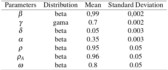
The prior distribution reflects the beliefs of the values of the parameters. A large standard deviation for this value means that there is little confidence in the a prior value used. Taking the worry of making a proper estimation: the distributions of the parameters; the mean values; and standard deviations, following values used in the literature.

Table 1 presents the a prior distribution of the parameters selected for the model of this work(Θ= (β, γ, δ, α, ρ, ρA,andω)).

Parameters Distribution Mean Standard Deviation

β beta 0,99 0,002

γ gama 0.7 0.002

δ beta 0.05 0.003

α beta 0.35 0.003

ρ beta 0.95 0.05

ρA beta 0.96 0.05

ω beta 0.8 0.05

Table 1: Prior distribution. Source: Prepared by the authors.

3.2

Posterior Distribution

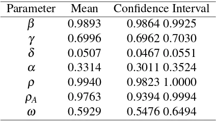
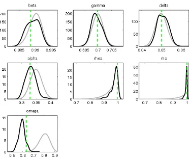
Table 2 presents the posterior distributions of the model and Figure 17compares the prior and posterior distributions.

The estimation results of this study followed the values obtained by the main DSGE literature. The value of the discount rate(β) estimated in this study was 0.9893. Rotemberg and Woodford (1997), Smets and Wouters (2003) and Juil-lard et al (2006) fix 0.99, while Christiano et al (2005) work 0.9926, among the articles related to Brazil: Kanczuk (2002) and Araujo et al (2006) use 0.99; while Ellery Jr et al (2010) choose 0.89; already Kanczuk (2004) chooses 0.98; Silveira (2008) works com 0.91; finally, Duarte and Carneiro (2001) fix 0.93.

7_{In Figure 1, the gray and black lines represent the prior and posterior distributions,}

We found the depreciation rate(δ)0.0507, while the international literature: Smets and Wouters (2003), Christiano et al (2005) and Juillard et al (2006) work with a depreciation rate of 0.025. While in Brazilian literature: Kanczuk (2002) uses 0.048; and Ellery Jr et al (2010) adopt 0.17.

The value found for the participation of private capital in the product(α)was 0.3314. While Kanczuk (2002) calibrates in 0.39, Ellery Jr et al (2010) think that this value is equal to 0.49 and Kanczuk (2004) uses 0.4, the same value that Duarte and Carneiro (2001).

The main parameter of this study is the population share of non-ricardian in-dividuals ((1−ω)). Who obtained value was 0.4071. Among the works related to Brazil: Reis, Issler, Blanco and de Carvalho (1998) found 0.8, already Cav-alcanti and Vereda (2011) worked with a range of values between 0.67 and 0.8, while Vereda and Cavalcanti (2010) and Monastier (2012) used the value 0.6. In foreign literature: Bosca et al (2010) used 0.5 for the Spanish economy; Camp-bell and Mankiw (1989) estimated this parameter for the G7 using OLS getting 0.616, 0.53, 0.646, 0.4, 0.553, 0.221 and 0.478 for Canada, France, Germany, Italy, Japan, England and United States, respectively; Gali et al (2007) worked with 0.5; Itawa (2009) found 0.25 for the Japanese economy; Mayer et al (2010) used 0.25 for the U.S. economy; and Stahler and Thomas (2011) obtained 0.44 for the Spanish economy.

Parameter Mean Confidence Interval

β 0.9893 0.9864 0.9925

γ 0.6996 0.6962 0.7030

δ 0.0507 0.0467 0.0551

α 0.3314 0.3011 0.3524

ρ 0.9940 0.9823 1.0000

ρA 0.9763 0.9394 0.9994

ω 0.5929 0.5476 0.6494

Figure 1: Prior and posterior distributions.

4

Results

the platform Dynare89.

4.1

Impulse-Response Functions

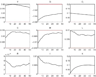
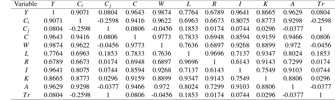
Figure 2 and Table 3 present the results for the shock in the payment of income transfer to non-ricardian. Note that a positive effect on output (Y), non-ricardian household’s consumption (Cj), aggregate consumption (C), labor supply (L), the

return on capital (R), investment (I) and the stock of capital (K). And a negative result in the ricardian individuals’ consumption (Ci), the level of wages (W) and productivity (A). Using Table 3, we can see two effects in opposite directions. The first relates to the negative effect of shockTrin the ricardian agents’ consumption, (Corr(Tr,Ci) =−0.2598), and on the other hand, a positive effect on labor supply

shock (Corr(Tr,L) =0.1853). These two effects will reverberate in the product,

and the negative result of the fall of the ricardian individuals’ consumption in the output (Corr(Ci,Y) =0.9071) is mitigated by the positive effect of labor supply

in the output (Corr(L,Y) =0.7764).

Other variables also exhibit high correlation with the product: 0.9643; 0.9874; 0.6789; 0.9641; 0.8665; and 0.9629. In relation to aggregate consumption, wage, return of capital, investment, capital stock and productivity, respectively. While the exogenous shock (Tr) has a low correlation with the product (0.0804).

Briefly, the shock in income transfer has a negative effect in the ricardian agents’ consumption, these, to try to maintain the level of consumption, increase

8_{Dynare is a software platform for the treatment of a broad class of macro models, in particular}

models of dynamic stochastic general equilibrium (DSGE) and overlapping generations (OLG). The models solved by Dynare include the hypothesis of rational expectations, but the Dynare is also able to handle models where expectations are formed differently: on one extreme, models where agents perfectly anticipate the future, at the other extreme, models where the agents have limited rationality or imperfect knowledge and thus form their expectations through a learning process. In terms of types of agents, it is possible to incorporate in Dynare: consumers; firms, government, monetary authorities, investors and financial intermediaries. Some degree of hetero-geneity can be accomplished by including several distinct classes of agents in each of the above categories of agents(Adjemian et al , 1996).

9_{The resolution models DSGE can be achieved using methods of disruption, which use a local}

Figure 2: Impulse-response functions for the shock in the payment of income transfers. Source: Prepared by the authors.

their labor supply, even with a fall in the wage level (Income effect). The overall effect of shock is positive, it is being able to keep the product above its steady state throughout the study period (fifty periods). Also, notice that the behavior of all variables is to stay away from the steady state, they are not showing a trend of return within the simulated period.10.

10_{Here is not being said that the variables will not return to steady states, but that these return}

Variable Y Ci Cj C W L R I K A Tr Y 1 0.9071 0.0804 0.9643 0.9874 0.7764 0.6789 0.9641 0.8665 0.9629 0.0804 Ci 0.9071 1 -0.2598 0.9416 0.9622 0.6963 0.6673 0.8075 0.8773 0.9298 -0.2598 Cj 0.0804 -0.2598 1 0.0806 -0.0456 0.1853 0.0174 0.0744 0.0296 -0.0377 1

C 0.9643 0.9416 0.0806 1 0.9773 0.7833 0.6948 0.8594 0.9159 0.9466 0.0806 W 0.9874 0.9622 -0.0456 0.9773 1 0.7636 0.6897 0.9268 0.8899 0.972 -0.0456

L 0.7764 0.6963 0.1853 0.7833 0.7636 1 0.9696 0.7137 0.9347 0.8024 0.1853 R 0.6789 0.6673 0.0174 0.6948 0.6897 0.9696 1 0.6143 0.9143 0.7299 0.0174 I 0.9641 0.8075 0.0744 0.8594 0.9268 0.7137 0.6143 1 0.7549 0.9103 0.0744 K 0.8665 0.8773 0.0296 0.9159 0.8899 0.9347 0.9143 0.7549 1 0.8806 0.0296 A 0.9629 0.9298 -0.0377 0.9466 0.972 0.8024 0.7299 0.9103 0.8806 1 -0.0377 Tr 0.0804 -0.2598 1 0.0806 -0.0456 0.1853 0.0174 0.0744 0.0296 -0.0377 1

Table 3: Correlation of Simulated Variables. Source: Prepared by the authors.

Conclusions

This work aimed to study the main Brazilian economic growth through a income transfer program. For this, we used the DSGE approach. The estimation of the pa-rameters was performed using the Bayesian methodology and analysis of results was done by impulse-response functions.

The results of the estimates followed, satisfactorily, the values found in the literature. The parameter that relates the population share of non-ricardian indi-viduals was slightly below the value found in the work related to Brazil. However, one can attribute this difference to the functional form of the consumption of these agents. In this work, we assume a form more restricted, since it believes that the non-ricardian agent only has transfers as revenue. Still, in section 3, one can no-tice the large variation of this parameter in the international literature DSGE.

The impulse-response functions showed positive responses to the variables:

Y, Cj, C, L, R, I, andK, and negative responses to the variables: Ci, W, andA.

The main result is that the ricardian agents’ consumption responds negatively to the shock, and these agents seek to compensate for this loss of utility increasing his labor supply. So even with this negative effect, the response of the economy to the shock is positive. Demonstrating that the introduction of the income transfer program brings positive returns for the whole economy, except for ricardian in-dividuals because consumption and wage level of these agents remains below its steady state throughout the simulation.

References

Adjemian, S., Bastani, H., Karamme, F., Juillard, M., Maih, J., Mihoubi, F., Peren-dia, G., Pfeifer, J., Ratto, M., and Villemot, S. (1996):Dynare: Reference Man-ual, Version 4.

Araujo, M., Bugarin, M., Muinhos, M., and Silva, J. R. (2006): The effect of adverse supply shocks on monetary policy and output. Banco Central do Brasil, Texto para Discussao, 103.

Bosca, J., Diaz, A., Domenech, R., Ferri, J., Perez, E., and Puch, L. (2010): A Ra-tional Expectations Model for Simulation and Policy Evaluation of the Spanish Economy. SERIEs, 1(1).

Brock, W., and Mirman, L. (1972): Optimal economic growth and uncertainty: The discounted case. Journal of Economic Theory, 4, 479 - 513.

Campbell, J., and Mankiw N. G. (1989): Consumption, income, and interest rates: Reinterpreting the time series evidence. NBER Macroeconomics Annual, MIT Press, pages 185 - 246.

Canova, F. (2007): Methods for Applied Macroeconomic Research. New Jersey: Princeton University Press.

Cass, D. (1965): Optimum growth in an aggregative model of capital accumula-tion. Review of Economic Studies, 32, 233 - 240.

Castro, J. A., and Modesto, L. (2010): Bolsa Familia 2003-2010: Avancos e De-safios. IPEA: Brasilia.

Cavalcanti, M. A. F. H., and Vereda, L. (2011): Propriedades dinamicas de um modelo DSGE com parametrizacoes alternativas para o Brasil. Ipea, Texto para Discussao, n 1588.

Christiano, L., Eichembaum, M., and Evans, C.. (2005): Nominal rigidities and the dynamic effects to a shock of monetary policy. Journal of Political Economy, 113, 1 - 45.

Coenen, G., and Straub, R.. (2004): Non-ricardian households and fiscal policy in an estimated DSGE modelo to the Euro Area. Mimeo.

Colciago, A..(2011): Rule of thumb consumers meet sticky wages. Journal of Money, Credit and Banking, 43, 325 - 353.

Colciago, A., Muscatelli, V. A., Ropele, T., and Tirelli, P.. (2006): The role of fiscal policy in a monetary union: Are national automatic stabilizers efective?

ECONSTOR, Working Paper, 1682.

Dallari, P.. (2012): Testing rule-of-thumb using irfs matching. Departamento de Econom ˜Aa Aplicada - Universidade de Vigo.

Diaz, S. O.. (2012): A model of rule-of-thumb consumers with nominal price and wage rigidities. Bando de La Republica - Colombia, Borradores de Economia, 707.

Duarte, P., and Carneiro, D.. (2001): Inercia de juros e regras de taylor: Explo-rando as funcoes de resposta a impulso em um modelo de equilibrio geral com parametros estilizados para o Brasil. Td 450, Departamento de Economia-Puc-Rio.

Ellery Junior, R., Gomes, V., and Sachsida, A.. (2010): Business cycle fluctuations in Brazil. Revista Brasileira de Economia, 56, 269 - 308.

Fernandez-Villaverde, J., and Rubio-Ramirez, J. F. (2004): Comparing dynamic equilibrium models to data: a bayesian approach. Journal Econometrics, 123(1), 153-187.

Fornero, J.. (2010): Ricardian equivalence proporsition in a NK DSGE model for two large economies: The EU and the US. Central Bank of Chile, Working Paper, 563.

Forni, L., Monteforte, L., and Sessa, L.. (2009): The general equilibrium effects of fiscal policy: Estimates for the euro area. Journal of Public Economics, 93, 559 - 585.

Furlanetto, F., and Seneca, M.. (2007)Rule-of-thumb consumers, productivity and hours. Norges Bank, Working Paper, 5.

Gali, J., Lopez-Salido, J. D., and Valles, J.. (2007) Understanding the effects of government spending on consumption. Journal of the European Economic As-sociation, 5(1), 227 - 270.

Ireland, P. N. (2004):A method for taking models to the data. Journal of Economic Dynamics and Control , 28(6), 1205-1226.

Itawa, Y.. (2009): Fiscal policy in an estimated DSGE model of the Japanese economy: Do non-ricardian households explain all? ESRI Discussion Paper Series, 216.

Kanczuk, F.. (2004): Choques de oferta em modelos de metas inflacionarias. Re-vista Brasileira de Economia, 58, 559 - 581.

Koopmans, T.. (1965): On the concept of optimal economic growth. The Econo-metric Approach to Development Planning, Amsterdam.

Kydland, F., and Prescott, E.. (1982): Time to build and aggregate fluctuations. Econometrica, 50, 1350 - 1372.

Johnson, D., Parker, J., and Souleles, J.. (2006): Household expenditure and the income tax rebates of 2001. American Economic Review, 90(2), 1589 - 1610.

Juillard, M., Karam, P., Laxton, D., and Pesenti, P.. (2006): Welfare-based mone-tary policy rules in an estimated DSGE model of the us economy. ECB, Working Paper, 613.

Lubik, T., and Schorfheide, F. (2003): Do central banks respond to exchange rate movements? a structural investigation. The Johns Hopkins Univer-sity,Department of Economics, Economics Work ing Paper Archive, 505 , 0-1.

Lubik, T., and Schorfheide, F. (2005): A bayesian look at new open economy macroeconomics. The Johns Hopkins University,Department of Economics, Economics Work ing Paper Archive, 521 , 0-1.

Mayer, E., and Stahler, N.. (2009): Simple fiscal policy rules: Two cheers for a debt brake!XVI Encuentro de Economia Publica.

Mayer, E., Moyen, S., and Stahler, N.. (2010): Fiscal expenditures and unemploy-ment: A DSGE perspective. ECONSTOR, Working Paper, E6 - V3.

Monastier, R. A.. (2012): O impacto de variaveis fiscais sobre o bem-estar na economia brasileira sob uma abordagem DSGE. Dissertacao, UFPR.

Motta, G., and Tirelli, P.. (2010): Rule-of-thumb consumers, consumption habits and the taylor principle. University of Milan - Bicocca, Working Paper Series, 194.

Ramsey, F.. (1927): A contribution to the theory of taxation. Economic Journal, 37(145), 47 - 61.

Ramsey, F.. (1928): A mathematical theory of saving. Economic Journal, 38(152), 543 - 559.

Reis, E., Issler, J. V., Blanco, F., and de Carvalho, L. M.. (1998): Renda perma-nente e poupanca precaucional: Evidencias empiricas para o Brasil no pas-sado recente. Pesq. Plan. Econ., 28, 233 - 272.

Rotemberg, J., and Woodford, M.. (1997): An optimization-based econometric framework for the evaluation of monetary policy. NBER Macroeconomics An-nual, 12, 297 - 346.

Schorfheide, F. (2000): Loss function-based evaluation of dsge models. Journal of Applied Econometrics, 15(6), 645-670.

Siveira, M. A.. (2008): Using a bayesian approach to estimate and compare new keynesian DSGE models for the Brazilian economy: the role for endogenous persistence. Revista Brasielira de Economia, 62, 333 - 357.

Smets, F., and Wouters, R.. (2003)An estimated dynamic stochastic general equi-librium model of the euro area. Journal of the European Economic Association, 1(5):1123 - 1175.

Stahler, N., and Thomas, C.. (2011): Fimod a DSGE model for fiscal policy simu-lations. Banco de Espana, Documentos de Trabajo, 1110.

Swarbrick, J.. (2012): Optimal fiscal policy in a dsge model with heterogeneous agents. Master thesis, School of Economics, University of Surrey.

Vereda, L., and Cavalcanti, M. A. F. H.. (2010): Modelo dinamico estocastico de equilibrio geral (DSGE) para a economia brasileira. Ipea, Texto para Discus-sao, 1479.