THE GENERALIZED GRADIENT, ITS COMPUTATION ASPECTS AND ITS RELATIONS TO THE MAXIMUM PRINCIPLE EUR 411 e

THE GENERALIZED GRADIENT,

'Mii·

F r a n c s 40, from : P R E S S E S ACADEMIQUES EURO-P E E N N E S — 98, Chaussée de Charleroi, Brussels 6. Please remit payments :

— to BANQUE D E LA SOCIETE G E N E R A L E (Agence Ma Campagne) — Brussels — account ... No 964.558,

- AMERICAN BANK AND T R U S T

York — account No 121.86,

II

giving the reference : « E U R 4 1 1 . e — The g e n e r a l i z e d ^ ; ^

Î

the maximum principle ».

This document w a s duplicated on the basis of the

mmm WSfâsSm m MmËmMî. mmèmm

¿ai:

EUR 411.e

EUROPEAN ATOMIC ENERGY COMMUNITY - EURATOM

THE GENERALIZED GRADIENT,

ITS COMPUTATION ASPECTS AND ITS RELATIONS

TO THE MAXIMUM PRINCIPLE

by

W.

DE BACKER

1963

Joint Nuclear Research Center Ispra Establishment - Italy

Scientific Data Processing Center - CETIS

CONTENTS

1. INTRODUCTION

2. STATEMENT OF THE PROBLEM

3. THE GENERALIZED GRADIENT AS A SPECIAL CASE OF THE

MAXIMUM PRINCIPLE

3.1 The optimal trajectory- completely lies in the

interior of G

3.2 The trajectory partly lies in the interior of

G and partly on the boundary of G.

3.3 The transversality conditions

3.1 Conclusions

4. THE STEEPEST DESCENT AS A SPECIAL CASE OF THE

GENERA-LIZED GRADIENT

5. COMPUTATIONAL ASPECTS OF THE GENERALIZED GRADIENT

6. EXAMPLE OF A GENERALIZED GRADIENT APPLICATION

7. APPLICATION FIELDS

THE GENERALIZED GRADIENT, ITS COMPUTATIONAL ASPECTS

AND ITS RELATIONS TO THE MAXIMUM PRINCIPLE

SUMMARY

The maximum principle and the related theorems of the Pontrya­ gin team lead to a generalization of the well­known steepest descent possible.

This generalization comprises the introduction of dynamic stresses.

For this reason the state vector no longer moves along the steepest descent, but the ^ ­ v e c t o r of the adjoint system does.

W i t h r e s p e c t t o t h e s i m u l a t i o n o f t h e d y n a m i c s t r e s s e s a n d t h e e l e g a n t t e c h n i q u e o f i m p l i c i t c o m p u t i n g o f L a g r a n g e m u l t i p l i e r s , t h e a n a l o g u e c o m p u t e r a p p e a r s t o b e a p p r o p r i a t e f o r g e n e r a l i z e d g r a d i e n t o p t i m i z a t i o n .

1. INTRODUCTION

We c o n s i d e r t h e p r o b l e m of m i n i m i z i n g a g i v e n f u n c t i o n F ( χ , . . . ,

χ 5 . . . , χ ) where t h e v a r i a b l e s χ ) a r e s u b j e c t t o c o n s t r a i n t s of t h e form:

One p o s s i b l e t e c h n i q u e f o r t h i s k i n d of p r o b l e m i s b a s e d upon t h e c o n ­

s t r u c t i o n of a s e t of d i f f e r e n t i a l e q u a t i o n s o f t h e s t e e p e s t d e s c e n t t y p e

f o r t h e v a r i a b l e s x ' . Pyne |_2J h a s done t h i s f o r l i n e a r programming

p r o b l e m s on t h e a n a l o g c o m p u t e r , b u t h i s method i s e q u a l l y v a l i d f o r

n o n l i n e a r o b j e c t i v e f u n c t i o n s and c o n s t r a i n t s . R e p r e s e n t i n g t h e whole

s e t of v a r i a b l e s χ by t h e v e c t o r x = ( x , . . , , x , . . . , χ ) t h e

s t e e p e s t d e s c e n t e q u a t i o n s can be w r i t t e n a s

m

¿ ï -

- k

g r a d F ( χ ) +/ k . g ^ ( x ) g r a d g ( x ) J ( 1 )

­ 2 ­

with: k. = 0 if gJ(x) ^ O

J i ( 2 )

k. = large and positive if g (x) > 0 »J

An additional aspect of these equations is the implicit computation of the functions k. g (χ) as approximations of the Lagrange multipliers for

i

g (χ) = 0. This is related to the theory of the penalty functions studied by Courant and Moser Í 3j · Indeed, relation ( 1 ) could have been written

= ­ k grad Ρ ( χ )

( 3 )

ui

J = 1

as

dx

d t

where Ρ (χ) i s a p e n a l t y f u n c t i o n

m

Ρ ( χ ) = F ( χ ) + j

which has to be minimized without additional constraints. The approxi­ mation is the better the more k. tends to infinity for g ( χ ) ^ 0.

J

It is obvious that the set of equations ( 1 ) and ( 2 ) or ( 3 )> ( 4 ) and ( 2 ) is not the only possible one describing trajectories of χ (t) ending at (at least a local) minimum of F (x). This means that addi­ tional constraints and even additional criteria with respect to the optimal trajectory could be satisfied before it is uniquely determined. These latent degrees of freedom make some generalizations possible. The maximum principle and other theorems of the Pontryagin team fll will permit us to analyse a related but more general problem and to define the con­

cept of generalized gradient.

2. STATEMENT OF THE PROBLEM

F (χ , . . ., χ , . . ., χ ) is a given function which has to be guided to its (local) minimum at some time t , taking account of following system of constraints.

We consider χ (t) to be a state vector x = ( x , . . , , x , . . . , x ) , belonging to a closed subset G of the n­dimensional state space and whose evolution is described by a system of ordinary differential

equations

3

-with f = (f , . . ., f , . . ., f ). In this system the control vector

u = (u , . . ., u ) has to be chosen as an element of the closed subset

U of the r­dimensional control space. The subset G is defined by

g

(x) < 0

j = 1, . . ., m

( 6 )

and the subset U is defined by

q

(u) ^ 0

1 = 1, . . ., s

( 7 )

We shall show that minimizing F (χ) by generalized gradient corresponds

to minimizing the functional

t+T

J (x) = F Γ χ (t + T)l - F Fx (t)] =

/ f° (χ, u) dt'

( 8 )

è

with

f° (χ, u ) = y ^ i g i

«

)

The initial condition χ of the optimal trajectory reduces to one point.

At every instant χ = χ (t). The final condition χ = χ (t + T) belongs

to the set of all possible x, reachable in a time Τ from t, with ad­

missible

We call this set R„ (t) and its boundary ρ jx (t + T)| = 0.

3. THE GENERALIZED GRADIENT AS A SPECIAL. CASE­OF THE MAXIMUM PRINCIPLE

).1. The optimal trajectory completely lies in the interior of G

Requiring that u (t) is piecewise continuous and that all f and all

^F/V

χ are defined and continuous on G χ U together with their partial

derivatives, we can apply the maximum principle for the problem de­

fined in § 2. By definition we have

Ή W

) f

( 10 )

¿~o ¿=1

­ 4 ­

- -

-^ - -t

st £r> - ¿ ( « *r, j-j )

Jx

-Knowing that /Γ is negative and constant this relation can be reduced to

d

(

^

γ

1 F

=

_ y

(

y

γ, ^

2L.

¿χ

¿, «

°)¿")¿-Calling / . + / c—r­ = / · WQ can write the Hamiltonian system as

>x

f o l l o w s /M

dx

7 > #

i

d t

_{3 % '}

/vi

ÍVí

~*>%

χ ­ ^ O /

d r i

- Σ T&'Ür

This formulation obviously corresponds to another problem, which has the same f' (x, u) as the original one of § 2, but with a different adjoint system ( γ . ·/ ψ. ) and with f = 0 . Such a problem has a

trivial solution. All admissible u g U satisfying the boundary con­ ditions are optimal. This is only possible if 3t = 0, which means

j . = 0 , indepondantly of U , initial or final conditions. For this ι

reason we have

Ί fa

°

­ 5 ­

3.2. The trajectory partly lies in the interior of G and partly on

the boundary of G.

Introducing the Lagrange multipliers for the boundary of G and the jump conditions for r at the junction points where the optimal trajectory reaches or leaves the boundary of G, we apply the

maximum principle for restricted state coordinates. A reasoning similar to that of § 3.1. leads to the relations ( 12 ) and ( 13 )· For simplicity we took m = 1 in relation ( 6 ).

γ

!?+

x

lz

r

-,

# . o

( ,

2 )

£>x ¿x

X = 0 for g (χ)

<

y~

^

·

its.

λ = ­

i ^ *

» s

for g (χ)

= 0

( 1 3 b)

Y ( ^ )

2

0 = 1

Relation ( 13 b ) satisfies the boundary condition (/, grad g) = 0 for g (χ) = 0 +)

3.3· The transversality conditions

Since <χ= 0 it finally turns out that the optimal control u has to be determined by the transversality conditions of the theorems of Pontryagin, stating that r(t ) , which corresponds in our problem to r ( t + T ) , has to be orthogonal to the set Ρφ(Ό of the final

events χ = χ ( t ) ■= χ ( t + Τ ) . Two possibilities have to be con­ sidered. They are illustrated in Fig. 1.

a) χ (t + T) lies in the interior of L (t). In this case the orthogonality condition can only be satisfied by

y

i (

f T > . g i

+

> ! £ )

l ( t + T )

. o

( 1 4 )

6

-This is true whatever be the value of T.

b) χ (t + T) lies on the boundary Ο [χ (t + T)] = 0 of ET(t),

Now we have

i>

"3

_ÌL,

^ <

'-^

^-(t

T)-/'^)x(t

,)

< ' 5 >

Fig. 1

3·4· Conclusions

1. With the generalized gradient it is no longer true that dx/dt = f (χ, u) moves along the steepest descent, but the vector jr

of the adjoint system takes over the same function.

2. Since the Hamiltonian is identically zero, the optimal control can only be determined by the transversality conditions and not necessarily in a unique way.

3. If the optimal trajectory χ (t) stops somewhere (dx/dt = θ) at a time f in a point χ (f)» it necessarily stops inside Rm (f). This means (cfr ( 14 )) that this point is a (local) optimum of F (x). The fact that the trajectory stops implies u = constant,

but not necessarily u = 0.

7

-Fig. 2

5· Whenever χ (t + Τ) lies on the boundary €>= O of R_ (t), the

trajectory can be determined by ( I5 )> the definition of

0 = 0 and the equations ( 7 ) giving the boundary of U. Indeed

these relations determine u (t) and L·. Examples will be given

in

§ 4

§

6. Whenever χ (t + T) lies in the interior of R„ (t) the trajectory

is not uniquely determined unless Τ =Δ t is arbitrarily small.

Indeed, the trajectory is composed of a sequence of initial conditions χ (t) of an optimization problem for t ^ t' ¿ t + T of which only the final condition is given by our optimization

criterion (8). In this case we propose a new optimization criterion.

t + T

■ / _{F (χ) dt' ( 16 )}

The problem will be subject of further study. Meanwhile the

difficulty will be bypassed by taking T arbitrarily small, which eliminates the optimization between t and t + T.

7. It should be noticed that the evolution of the system only takes

accoxmt of the direction of the vector (grad F + ,Χ grad g ) and not of its magnitude. The speed of evolution is more closely

related to the system of dynamical constraints ( 5 ) an(i the

8

-8. While optimizing we have to take account of the values of F (χ)

only for χ in the interior of R,p(t). Outside this region F (χ)

is completely ignored. It looks as if the optimizing system has

a limited "horizon" of information around the moving point χ (t)

and which is defined by Η

(ΐ). If the trajectory stops at a

local optimum, the optimizer never finds a possibly higher

optimum if this lies outside its horizon. The probability of

staying at a local optimum obviously grows with decreasing Τ

and becomes a certainty for Τ arbitrarily small. The concept

of the horizon of an optimizing system seems to be realistic.

Indeed, the ability of predicting and interpreting all possible

events within some time period Τ is linked to a degree of complexit

which is limited for most technologically realizable optimizing

systems.

4. TEE STEEPEST DESCENT AS A SPECIAL CASE OF THE GENERALIZED GRADIENT

We consider the problem of § 2 with the following restrictions:

Τ =

A

t = arbitrarily small

f

= u

i = 1, . . ., η ( 17 )

q (u) =

¿ J u

)

- 1 ^ 0

( 18 )

6=1

By ( 18 ) U is represented by a unit hypersphere in the n­dimensional

state­space. It follows immediately that R

(t)' too is a hypersphere

Δ

t

with r a d i u s

Δ

t and t h a t f o r x ( t + Z l t ) o n the boundary

P= 0 we

have

"ox

"dx

^

) /

7>χ

^

)

/

- J

= ( 2 / 4 t ) u

Knowing that for χ (t + 4 t ) on D = 0, u i s o n q ( u ) = O w e can

calculate

­ 9 ­

Since

h,

is negative for a minimizing problem we have the following

final solution:

If­ = 0

for grad F +

\

grad g = 0

( 19 )

d. χ

Il = ­ k (grad F +

\

grad g)

( 20 )

with

X = ( 13 a ) and ( 13 b')

■K

k =

2A

41

­1­1/2

.<__ ¿)x

2>χ

( 21 )

Relations ( 19 ) and (­*?0 ) obviously are equivalent to ( 1 ) for

m = 1. The only points meriting some comment are k and A · As stated

already in the introduction k. g (χ) (j = 1) is nothing but an

approximation of the Lagrange multiplier

\

, generated by implicit

computing. As far as k is concerned, in relation ( 20 ) it has been

taken for the highest possible speed of χ up to the endpoint. At the

endpoint however, ( 19 ) is necessary since ( 20 ) becomes undeter­

mined. In relation ( 1 ) k has not yet been specified. The only im­

portant restriction on k is that it is a scalar, which is the case

in ( 1 ) as well as in ( 20 ).

To resume, it has been shown that for the steepest descent not only

j .

but also dx /dt is directed along (grad F + ,λ grad g). This is

true because Τ =

Δ

"t and

D

lx (t +

Δ

t)l = 0 is a hypersphere.

5. COMPUTATIONAL ASPECTS OF THE GENERALIZED GRADIENT

On condition that grad F (χ) and grad g (x) have sufficiently simple

analytical expressions (or some simple analytical approximation,

preferably linear, quadratic or third order polynomials) the

equations ( 1 ) can be programmed without difficulty for analog and

digital computers. In most cases the same is true for the generalized

gradient if we take Τ =

Δ\

t. Especially when the set of equations ( 5 )

constitutes a complicated, high order, non­linear dynamical system the

10

-We draw special attention to the implicit computing of the Lagrange multipliers by k . g (χ) or the equivalent technique of the penalty functions. This technique is extremely simple and well adapted for programming on analog computers,., because of the continuous repre­ sentation of the variables on the computer. B.ut equally for digital computers the technique seems to have considerable advantages with respect to the direct computation of the Lagrange multipliers by relation ( 1 3 a , b ) . The accuracy of the approximation technique can be studied in terms of constraint "violations", corresponding to the maximum positive values of g (x). These violations are roughly proportional to λ./k., a ratio which tends to zero with growing k.. For large k. however, difficult convergence problems

J J

in digital computers may arise. Even with the analog computer, in spite of its continuous representation, stability may become an embarrassing problem, since the stability is more strongly related to the structure of equations ( 5 ) an(i ( 7 )· Introducing additional

damping forces for g ( x ) ^ 0 or nonlinear functions instead of

-j '

constant k s is very useful, but their influence upon the accuracy of the optimal trajectory still has to be examined carefully.

The simulation of IT on a digital computer generally poses no difficult problems. On the analog computer it can be done in several ways. If possible the use of limiters is the most practical one. This is especially true for hyperparallelopipeds. A more general technique is once more the introduction of Lagrange multipliers y for q (u) = 0, which have to be computed again in the same way as the

X 's. Since u (t) can move in U without friction and without inertia, new stability problems add to the already discussed ones. They very often can be solved by a more realistic interpretation of the under­

lying physical phenomena.

Whenever grad F (χ) and grad 'g (x) have no simple analytical ex­ pression all hope should not bo lost. Modern perturbation techniques and sensitivity analysis are often very useful and easily pro­

grammable tools for estinuiting cumplicated gradients. This is especially the case for iteration procedures of the gradient type for solving two point boundary problems and parameter optimizations

­ 11

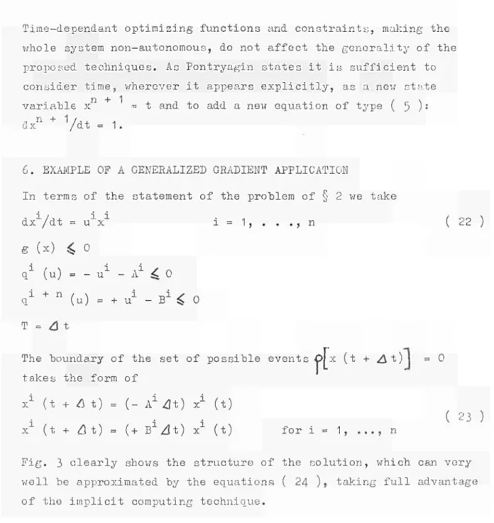
Time­dependant optimising functions and constraints, making the whole system non­autonomous, do not affect the generality of the proposed techniques. As Pontryagin states it is sufficient to consider time, wherever it appears explicitly, as a new state variable χ ­ t and to add a new equation of type ( 5 ):

, η + 1 /, , .

dx /dt = 1 .

6. EXAMPLE OF A GENERALIZED GRADIENT APPLICATION

In terms of the statement of the problem of § 2 we take

dx /dt = u"x i = 1, . . ., n

ë

(χ) i o

q1 (u) = ­ u1 ­ Ai ^ 0

¿

(u)

= +

u

­

B

< 0

τ =

Δ

t

The boundary of the set of possible events θ\ χ (t + Δ t) j

takes the form of

x

(t +

¿\

t) = (­ A

¿it) x

(t)

x

( t + < u t ) = ( + B

d t ) x

( t )

for i = 1, ..., η

= 0

22 )

( 23 )

Fig. 3 clearly shows the structure of the solution, which can very well be approximated by the equations ( 24 ) , taking full advantage of the implicit computing technique.

4

°

q>o

­ 12

dx

dt ­ k χ grad F (χ) + ^ g (χ) grad g (x) ( 24 )

with: ­ Αχ ^ dx/dt <¡ Bx

k and k large and positive, but k = 0 for g (χ) ^ 0.

A and Β are constant vectors with coordinates A and Β , representing the edges of the hyperparallelopiped U.

The larger k and k the better the accuracy, but the more critical the stability of dx/dt whenever it lies between ­Ax and Bx. This particu­ larly happens on the boundary g (χ) = 0 (see fig. 3 ) .

The analog computing diagram takes the form of Fig. 4.

+25

(Λ

X r O

-A'

o F&J

k± γΟ-J grad

γ&)

13

-7. APPLICATION FIELDS

Tho most important class of engineering applications probably is the optimization of industrial production processes for which the slow variation of the properties of the process constitutes a system of dynamical constraints of type ( 5 )> a n¿ for which a certain profit

function corresponding to the quality of the final product, the pro-duction costs or some other criterion can be fixed |_6J.

Another interesting field would be the study of macro-economic structures, Indeed, the generalized gradient opens the possibility of integrating the laws of economic growth and economic optimization in one model.

ACKNOWLEDGEMENTS

14

-REFERENCES

Γ1Ί L. S. Pontryagin, V.G. Boltyanskii, R.V. Gamkrelidze,

E.F. Mishchenko: "The Mathematical Theory of Optimal Processes", John Wiley & Sons, New York," 1962.

J 2 J L.B. Pyne: "Linear Programming on an Electronic Analogue Computer", Communication and Electronics, 1936, 24: pp. 139 - 143«

Γ3Ι H.J. Kelley: "Method of Gradients" pp. 213 - 215, in "Optimi­ zation Techniques" (G. Leitmann, ed), Academic Press, New York, 1962.

I 4 I W. Brunner: "An Iteration Procedure for Parametric Model Building and Boundary Value Problems", Proc. Western Joint Computer Con­ ference, Los Angeles, Part 12, pp. 519 - 533«

I 5 L.W. Neustadt: "Applications of linear and non-linear Programming Techniques", Proc. 3rd Int. Analogue Computation Meetings, I96I, Presses Acad. Eur., Brussels, Sect. B 1, pp. 197 - 200.

Ï U R 4 1 1 . e

ΓΗΕ GENERALIZED GRADIENT, ITS COMPUTATIONAL ASPECTS AND ITS RELATIONS TO THE MAXIMUM PRINCIPLE by W. DE BACKER.

European Atomic Energy Community — EURATOM l'oint Nuclear Research Center

[spra Establishment — Italy

Scientific Data Processing Center ­—■ CETIS

rext distributed at the IFAC­Congress, Basel (Switzerland) — 27 August ­ 4 September 1963

Brussels, February 1964 ■—■ pages 14 ­—■ figures 4

The maximum principle and the related theorems of the Pontryagin team make some generalizations of the well­known steepest descent possible. This generalization comprises the intro­ iuction of dynamical constraints. For this reason the state vector io longer moves along the steepest descent, but the τ ­vector of the adjoint system does. With respect to the simulation of the dynamical ;onstraints and the elegant technique of implicit computing of Lagrange multipliers, the analog computer seems the indicated one for generalized gradient optimization.

E U R 4 1 1 . e

ΓΗΕ GENERALIZED GRADIENT, ITS COMPUTATIONAL ASPECTS AND ITS RELATIONS TO THE MAXIMUM PRINCIPLE by W. DE BACKER.

E\iropean Atomic Energy Community ­— EURATOM Joint Nuclear Research Center

Ispra Establishment ·— Italy

Scientific Data Processing Center — CETIS

r e x t distributed at the IFAC­Congress, Basel (Switzerland) — 27 August ­ 4 September 1963

Brussels, February 1964 — pages 14 — figures 4

m

m

iVlGËBM

û ¡irti"*'» Γ : Ui Ι1?» «ί jtttj^H