Contribution in Information Signal Processing for Solving State Space Nonlinear Estimation Problems

(1)

http://dx.doi.org/10.4236/jsip.2013.44048

Contribution in Information Signal Processing for Solving

State Space Nonlinear Estimation Problems

Hamza Benzerrouk1*, Alexander Nebylov2, Hassen Salhi1*

1_{SET Laboratory (Systèmes Electriques et Télecommande) of Electronic, Department of Saad Dahlab, University of Blida, Blida,} Algeria; 2_{International Institute for Advanced Aerospace Technologies, Saint-Petersburg State University of Aerospace} Instrumenta-tion, Saint Petersburg, Russia.

Email: *_{hb.iiaat@gmail.com, nebylov@aanet.ru,}*_{hassensalhi@yahoo.fr}

Received May 12th_{, 2013; revised September 30}th_{, 2013; accepted October 8}th_{, 2013}

Li-cense, which permits unrestricted use, distribution, and reproduction in any medium, provided the original work is properly cited.

ABSTRACT

In this paper, comprehensive methods to apply several formulations of nonlinear estimators to integrated navigation problems are considered and developed. The problem of linear and nonlinear filters such as Kalman Filter (KF) and Extended Kalman Filter (EKF) is stated. Analog solution which is based on fisher information matrix propagation for linear and nonlinear filtering is also developed. Additionally, the idea of iterations is included through the update step both for Kalman filters and Information filters in order to improve accuracy. Through this development, two new for-mulations of High order Kalman filters and High order Information filters are presented. Finally, in order to compare these different nonlinear filters, special applications are analyzed by using the proposed techniques to estimate two well-known mathematical state space models, which are based on nonlinear time series used to apply these estimation algorithms. A criterion used for comparison is the root mean square error RMSE and several simulations under specific conditions are illustrated.

Keywords: Kalman Filter; Information Filter; Extended Kalman Filter; Extended Information Filter; 2nd Order Kalman Filter; 2nd_{Order Information Filter}

1. Introduction

Different kinds of filters exist and were developed in order to ensure high quality measurement in input-output systems and permit more accurate control system in sev-eral fields such as in Aerospace, for aircraft’s navigation, ship, spacecraft, tracking etc. Kalman filter (KF) was firstly derived from using orthogonality principle and presented in [1-3]. Generally so-called filter or/and estimator, is/are one of several techniques of estimation based on LMMSE (Linear Minimum Mean Square Error) [4]. In 1970, Kalman and Bucy introduced extended Kalman filter for nonlinear estimation. Actually this kind of filter is called standard local filter and is based on approxima-tion of nonlinear funcapproxima-tions by Taylor series. The most common filter in the field of engineering and aerospace especially, is the extended Kalman filter. These local standard filters also contain the second order Kalman filter and the iterated filter. Other kinds of nonlinear

filtering algorithms exist but are not treated in this paper [5]. The most interesting and main idea introduced in this paper is to use the parallel solutions to Kalman filter and standard local filters which are based on the Fisher In-formation Matrix propagation [6,7]. It is analog to Kal-man technique but is more efficient and robust to several constraints. The main idea is to use the inverse matrix lemma to develop analog estimator to Kalman filter with less computational time. These filters are more efficient when the number of the input is more than the dimension of the state vector. In this paper, we introduced classic information filters for linear and nonlinear filtering problem. Behind this was explored in our solution, the efficiency includes iterations through the updated step of the different algorithms [8]. Two new formulations are presented such as the iterated second order Kalman filter and the second order information filter followed by the second order Iterated Information filter. So, generally the step of initialization is the main important in nonlinear filtering and we propose to use the information filters to

(2)

solve the problem of initialization. Of course, informa-tion filters present several other advantages when the state space model input is a combination of several sen-sors as in data fusion or multi-sensen-sors fusion, it was proven that comparing with Kalman filter and extended Kalman filter both for linear and nonlinear case, the in-formation filters are more easy to implement in real time application with multiple information combination [9-12]. We apply these different nonlinear filters to dynamical state models such as references. It is expected that this work could serve in investigate integrated navigation system INS (Inertial navigation System)/GNSS (Global Navigation by Satellite System) problems, in order to show possible application in the field of aerospace.

2. Kalman Filter and Nonlinear Filtering

If the system is linear and the statistical distribution is Gaussian, then the Bayesian prediction and update equa-tion can be solved analytically. The system is completely described by the Gaussian parameters such as mean and covariance and this filter is called the Kalman filter [13]. As a discrete statistical recursive algorithm, Kalman fil-ter provides an estimate of the state at time k given all

observations up to time k and provides an optimal

mini-mal mean squared error estimate of these states.

Process Model: A linear dynamic system in discrete time can be described by

1 . ₀

.

k k k k

x F x w k z H x v

  





  

 (1)

Kalman filter is usually called as the optimal filter in the case of linear assumption and white Gaussian noises both in state and in measurement equations.

2.1. Extended Kalman Filter

In most real applications the process and/or observation models are nonlinear and hence linear Kalman filter al-gorithm described above cannot be directly applied. To overcome this, a linearised Kalman filter or Extended Kalman Filter (EKF) can be applied which are estimators where the models are continuously linearized before ap-plying the estimation techniques [14].

However, in most practical navigation applications, nominal trajectory does not exist beforehand. The solu-tion is to use the current estimated state from the filter at each time step k as the linearization reference from which

the estimation procedure can proceed. Such algorithm is called extended Kalman filter. If the filter operates prop-erly, the linearization error around the estimated solution can be maintained at a reasonably small value [15-17]. However, if the filter is ill-conditioned due to modeling

errors, incorrect tuning of the covariance matrices, or initialization error, then the estimation error will affect the linearization error which in turn will affect the esti-mation process and is known as filter divergence. For this reason the EKF requires greater care in modeling and tuning than the linear Kalman filter. Let us describe bel-low the algorithm of EKF [18]: based on state space model as:

 

1 .

0 .

k k k k

x f x w k z h x v



  

 _



 

 (2)

and on the linearization using taylor approximation at the first order we get the state space model given in [19].

 

k

F  is the Jacobian matrix of f_k

 

 and H_k

 

 is

the Jacobian matrix of hk

 

 .

Initialization:

0 ˆ

x et P₀. (3)

Prediction:

 

1/

T

/ 1 1

ˆ ˆ

k k k k

k k k k k k k k

x f x

P F x P F x



 



Q

  (4)

Update:























T T

/ 1 / 1 / 1 / 1 / 1

1

/ 1 / 1

/ 1 / 1 / 1

ˆ ˆ ˆ

ˆ 1;

k k k k k k k k k k k k k k

k

k k k k k k k k

k k k k k k k k k

K P H x H x P H x R

x x K Z h x P P K H x P K K

   



 

  



 _



 

  _  _

 

 



(5)

The meaning of the extended Kalman filter can be un-derstudied by appreciating the same equation of gain calculation as in the Kalman filter at the difference that in the nonlinear filtering, EKF is sub-optimal filter.

2.2. Iterated Filter

One can distinguish the importance of the two different steps; prediction and update, it allows to observe the ef-fect of new information given by the measurements in the filtering step. Let us focus on the estimation of the mean and the covariance of the state vector. In Equation (5) it is clear that xˆ_k contains more information about

k

x than xˆ_k. Nonetheless, the linearization was made in

ˆk

x. This fact is used and the linearization can be made in

the kth step again but this time in xˆk. This provides a new value of estimates and such a procedure may be re-peated as long as a difference between two subsequent estimates is lower than a specified . Thus, the follow-ing equations will be implemented usfollow-ing the iterated form: _ˆ1 _ˆ

k k

(3)

   

 





 

1

T T

/ 1 / 1

1

/ 1 / 1

1

/ 1 / 1

ˆ ˆ ˆ

ˆ

i i i

k k k k k k k k k k k k

i i

k k k k k k k k

i i

k k k k k k k k

K P H x H x P H x R x x K z h x

P P K H x P

           _     _  _     _ (6)

The iteration is stopped if _ˆi1 _ˆi

k k

x x I with 0;

and the value i + 1, i.e. the time instant of iteration, is

denoted as imax. It is not possible to use the same iteration formulation for the prediction step because the prediction utilizes no new information from reality. So, the relation of prediction step is the same as in the extended Kalman filter. So,

 

1/

ˆ_k _k _k ˆ_k

x_  f x (7)

 

T

/ 1 ˆ 1 ˆ

k k k k k k k k

P  F x P F x 

i

Q (8)

where ˆ ˆmax

k k

x x and _P _Pimax .

k k

All the previous relations define the iterated filter which is an improvement of the extended kalman filter and improves local approximation for filtering estimate calculation. On the other hand, it is again local approxi-mation and convergence of the estimate is not guaranteed as well.

2.3. 2nd Order Kalman Filter

In this part, another alternative of the extended Kalman filter is presented and will be used in simulations. Based on the Taylor series but used to the second term, let us consider the following approximations:

 

 







T 2





2

ˆ ˆ ˆ

1 _ˆ _ˆ

2 k

k k k k k k k k

k

k k x k k

k

h x h x H x x x

h

x x x x

x               (9)

where ˆxk, correspond to the approxima-tion used for the extended Kalman filter.

 

,

k k

h  H 

The dimension of the vector function hk

 

 is nz and the dimension of the state vector xkis nx.

Then, the new approximation can be written such as described by:

 

ˆ

 

ˆ ˆ



1

2

k k k k k k k k k

h x h x H x x x  h (10)

Because of the second order terms in (10), analytical computation of the filtering step is not possible, so, we can solve this problem by replacing the quadratic form by its mean and we obtain then:





T









ˆ ˆ ˆ

ik k k ik k k k ik aik

h  x x M x x tr P M h ;

Let us write: hak  ha k1 ,ha k2 , , han k_z T and then, we obtain also:

 

ˆ

 

ˆ ˆ



k k k k k k k k ak

h x h x H x x x h ;

From this result, we can learn that it is a linear function

of xk, as all the remaining terms are known in the (k−1)th step. Thus we obtain the following integration equations:

 



 



 

T T 1 T T 1

ˆ ˆ ˆ ˆ ˆ

ˆ

ˆ ˆ ˆ

ˆ

k k k k k k k k K k

k k k k ak

k k k k k k k k k k

k k k

x x P H x H x P H x

R z h x h

P P P H x H x P H x

R H x P

           _    _   _          _     (11)

It is possible to observe that the innovation sequence is different from the one of the extended Kalman filter. Now, to compute the prediction step, it is possible repeat the same steps as for the update formulation and we ob-tain as bellow:

 

ˆ

 

ˆ ˆ



1

2

k k k k k k k k k

f x  f x F x x x  f ;

By computing means of the nonlinearities, it is possible to write: faik tr P N



k ik



&

T 1 , 2 , , x

ak a k a k an k

f  f f  f _ ;

Finally, we get:

 

ˆ

 

ˆ ˆ



x k k k k k k k ak

f x  f x F x x x  f ;

and we obtain:

 

1

T 1

ˆk k ˆk ak

k k k k k k

x f x f

P F x P F x Q



  

   _k; (12)

The equation of the Covariance integration is the same as in the extended Kalman filter, with different prediction step adding fak. So, the Equations (16) and (17)

repre-sent the second order filter.After describing the different nonlinear approximation used usually in nonlinear filter-ing , let us pass to the second kind of filters which are the information filters both for linear and nonlinear case, let us describe the information filter [20] and the extended information filter [21,22], then novel formulations will be developed.

3. Information Filter and Nonlinear

Information Filters

The information filter is mathematically equivalent to the Kalman filter except that it is expressed in terms of measures of information about the states of interest rather than the direct state and its covariance estimates. Indeed, the information filter is known to have a dual relationship with the Kalman filter. If the system is linear with an assumption of Gaussian probability density distributions, the information matrix Y k k



/



, and the information state estimate y



k k/



, are defined in terms of the in-verse covariance matrix and state estimate.



_/



1



_/

(4)



k k/



Y k k x k k



/

 

y /



(13) When an observation occurs, the information state contribution i(k) and its associated information matrix I(k)

are given by the following expressions:

 

T

 

1

   

k H k R k z k

i ; (14)

 

_k __HT

 

_{k R}1

   

_{k H k}

I (15)

By using these variables, the information prediction and update equation can be derived from Kalman filter.

Prediction: The predicted information state is obtained by pre-multiplying the information matrix

in Equation (22) and by representing it in information space,



/ 1

Y k k







 





    

/ 1 / 1 / 1

/ 1

y k k L k k y k k Y k k B k u k

   

  (16)

where the information propagation coefficient matrix (or the similarity transform matrix) L



k k/ 1 is given by



_/ ₁





_/ ₁

   

1 _/ ₁

L k k Y k k F k Y k k (17)

The corresponding information matrix is obtained by taking the inverse of Equation (18) and by representing it in information space,









  

1



/ 1 / 1

/ 1

L k k Y k k F k Y k k

  

  (18)

Estimation: The update procedure is simpler in the information filter than in the Kalman filter. The observation update is performed by adding the information contribution from the observation to the information state vector and its matrix:



/





/ 1

 

y k k  y k k i k (19)



/





/ 1

 

Y k k Y k k I k



(20) If there is more than one observation at time k, the

in-formation update is simply the sum of each inin-formation contribution to the state vector and matrix,











1

/ / 1 n j

j

y k k y k k i k



  



; (21)











1

/ / 1 n j

j

Y k k Y k k I k



  



; (22)

where n is the total number of synchronous observations

at time k.

Note: As the information matrix is defined like the inverse of the covariance matrix, the information filter deals with the “certainty” rather than “uncertainty” such as in Kalman filter. Furthermore, given the same number of states, process and observation models, the computa-tional complexity of the information filter and the

Kal-man filter are comparable. The update stage in the in-formation filter is quite simple however the prediction stage is comparatively complex, which is exactly oppo-site in the Kalman filter.

However both filters can show different computational complexity depending on the dimension of the state and observations. If the number of observations increases, as in the case of the multi-sensor systems, the dimension of the innovation matrix of the Kalman filter increases as well, and the inversion of this matrix becomes computa- tionally expensive. In the information filter, however, the information matrix has the same dimension of the state and its inversion is independent to the size of observations. This means that the information filter is an efficient algorithm when the dimension of observations is much greater than that of the state, thus, they are more suitable in complex data fusion problems based on multiple sensors.

In addition, the information filter can perform a synchronous update from multiple observations in contrast to the Kalman filter. The reason is that the innovations in the Kalman filter are correlated to the common underly- ing state while the observation contributions in the information filter are not. This makes the information filter attractive in decentralizing the filter. Finally, the information filter can easily be initialized to zero information.

Extended Information Filter

The extended information filter can also be derived for the nonlinear process/observation model defined in Equa- tions [22].

Prediction: The predicted information vector and its information matrix are obtained by using the Jacobians of the nonlinear process model



/ 1





/ 1





/ 1 ,

  

,0



y k k Y k k f x k k u k (23)





  



 

   

 

1 T

/ 1 x 1/ 1 x

Y k k f k Y k k f k f_ k Q k f_ k



 

  _   



  _ (24)

Estimation: When an observation occurs, the information contribution and its corresponding matrix are:

 

   

 

  



1

T T

/ 1

x v v

x

i k h k h k R k h k k h k x k k





 

  _  _

_    _ (25)

 

_T

 

   

_T

 

1

 

x v v x

I k  h k _h k R k h k _ h k (26)

where the innovation vector is also computed as in the EKF

 

k z k

 

h x k k



/ 1 ,0



    (27)

(5)



/





/ 1

 



y k k  y k k i k (28)



/





/ 1

 

Y k k Y k k I k



(29)

In practice, the EKF and EIF are considered as the most useful filters.

4. Contribution in Information Nonlinear

Filtering

In this section, new filters based on the presented techniques are introduced, using iterations to improve the second Order Kalman filter and the extended Information filter, these filters were called: Iterated 2nd_{Order Kalman} Filter and Iterated Extended Information filter, we applied these two new formulation in simulations and it is expected to have a good results. The main is to proof that the iteration can be also applied to High order Kalman filter and can improve the accuracy of the Extended information filter. Of course, the computational time will increase instead of more accuracy.

The second contribution in his paper is to extend information filter to the second order based on the 2nd_order Kalman filter and to apply also the iterations through the update of the new filter in order to improve its efficiency. These algorithms are called 2nd_{Order Information filter} and Iterated 2nd_{Order Information filter. Let us begin by} describe the Iterated 2nd_{order Kalman filter , the iterated} Extended Information filter, the 2nd_{order Information} filter and finally, the Iterated 2nd_{order Information filter.}

4.1. Iterated 2nd Order Kalman Filter

The iterated filter from the previous section represents a way to improve the point of linearization of the nonlinear function and the second derivation of this function. In this part, another alternative of the extended Kalman filter is presented and will be used in simulations. Based on the Taylor series but used to the second term, let us consider the approximations given in the Equation (9). Where

 

k

h 

ˆ_k

x, h_k

 

 , H_k

 

 correspond to the ap-

proximation used for the extended Kalman filter. The dimension of the vector function h_k

 

 is nz and the dimension of the state vector xk is nx.

The same assumption such as made in the 2nd_order Kalman filter is considered at expect of introducing the iterations through the update step of the algorithm. So, the same idea of the iterated filter will be applied again.

Thus we obtain the integration equations given by Equation (15). It is proposed to transform this step by introduce iterations till the error between subsequent estimates will be less then specified error minimum limit.

So, the new update is given bellow: ˆ1 ˆ

k k

X X and

.

1

k k

P P i

For 1, 2,3,

   

 

   

 

1

1 T T

1

1 T T

ˆ ˆ ˆ ˆ ˆ

ˆ

ˆ ˆ ˆ

ˆ

i i i i

k k k k k k k k K k k

k k k ak

i i i i

k k k k k k k k k k k

i k k

x x P H x H x P H x R z h x h

P P P H x H x P H x R H x P

 

 

  

  _  _

  

_   _

 

  

  _  _

 

(30)

If _ˆi1 _ˆi

k k

x x I with  0. Then stop the itera-

tions, else, continue, end.

So, one can observe that the update equations are the same such as in the iterated Kalman filter according to the covariance integration but is different in state estimation due to the correction term in the innovation.

Now, to compute the prediction step, it is possible to repeat the same steps as for the update formulation and we obtain the following equation:

 

ˆ

 

ˆ ˆ



1

2

k k k k k k k k k

f x  f x F x x x  f

By following exactly the same steps such as in the 2nd order Kalman filter; we finally obtain:

 

1

T 1

ˆk k ˆk ak

k k k k k k

x f x f

P F x P F x Q



  

   _k; (31)

where _ˆi _ˆimax

k k

x x and i imax.

k k

P P

The equations of the state and Covariance integration are the same such as given in the 2nd_{order Kalman filter.} So, the Equations (37) and (38) represent the second or-der filter.

4.2. Iterated Extended Information Filter

The extended information filter can also be derived from the nonlinear process/observation model equations.

Prediction: The predicted information vector and its information matrix are obtained by computing the Jaco- bian of the nonlinear process model given in the Equa- tion (2).

Estimation: When an observation occurs, the information contribution and its corresponding matrix are written such as below:

For 1, 2,3,j 

 

   

 

  



1

T T

/ 1

j

j x v v

x

i k h k h k R k h k k h k x k k





 

  _  _

 

_    _

 

_T

 

   

_T

 

1

j x v v

(32)

 

j xj

I k  h k _h k R k h k _ h k

(33) where the innovation vector is also computed like in EKF

 

k z k

 

h x k k



/ 1 , 0



   



(34)

(6)

information state vector and matrix such as in linear in-formation filtering:



/





/ 1





j j j



y k k y k k i k (35)



/





/ 1





j j

Y k k Y k k I_j k



(36)

when

1

1 1

j j

k k

I Y  Y  ,

where 0, End.

4.3. 2nd Order Information Filter

Again, the same technique used in the extended information filter is used, based this time on the second order approximation of the state and the covariance using the corrected innovation.

Prediction: The predicted information vector and its information matrix are obtained by computing the Jaco- bians of the nonlinear process model and the corrected form of the predict state in the second Kalman filter:



/ 1





/ 1





/ 1 ,

  

, 0



ak

y k k Y k k f x k k u k  f



(37)





  



 

   

 

1 T

/ 1 x 1/ 1 x



 

  _   



   _ (38)

where fak is the second order term used to correct the

predict state calculated in the previous section according the 2nd_{Order Kalman filter.}

 

   

 

  



1

T T

/ 1

x v v

x

i k h k h k R k h k k h k x k k





 

  _ 

_   



 (39)

 

_T

 

   

_T

 

1

 

x v v x

I k  h k _h k R k h k _ h k (40)

where the innovation vector is also computed as in the 2nd_{order KF}

 

k z k

 

h x k k



/ 1 ,0



hak

     (41)

It is possible to observe that the innovation sequence is the same such as in the 2nd_{KF but is more accurate than} in the Extended Information Filter (EIF). These information contributions are again added to the information state vector and information matrix:



/





/ 1

 



y k k y k k i k (42)



/





/ 1

 

Y k k Y k k I k



(43)

Let us now consider the 2nd_{Order Information Filter} and compare with the 2nd_{Order Kalman filter through}

simulations in the last section.

4.4. Iterated 2nd Order Information Filter

The same philosophy such as in the previous section is used. Iterations are introduced through the update step, in order to increase accuracy of linearization and the second derivation.

Prediction: The predicted information vector and its information matrix are obtained by using the Jacobians of the nonlinear process model and the corrected form of the predict state in the second Kalman filter:



/ 1





/ 1





/ 1 ,

  

, 0



ak



y k k Y k k f x k k u k  f

(44)





  



 

   

 

1 T

/ 1 x 1/ 1 x



 

  _   



   _ (45)

where fak is the second order term used to correct the

predict state calculated in the previous section according the 2nd_{Order Kalman filter.}

For l1, 2,3,

 

   

 

  



1

T T

/ 1

l

l x v v

x

i k h k h k R k h k k h k x k k





 

  _  _

 

_    _

 

_T

 

   

_T

 

1

l l

l x v v

(46)

 

x

I k  h k _h k R k h k _ h k (47)

where the innovation vector is also computed such as in the EKF

 

k z k

 

h x k k



/ 1 , 0



h_ak

     (48)

These information contributions are again added to the information state vector and matrix as in the linear in-formation filter



/





/ 1

 

l l l



y k k y k k i k (49)



/





/ 1





l l l

Y k k Y k k I k



(50)

when

1

1 1

l l

k k

I Y  Y 

where 0, End.

(7)

ally based on nonlinear filtering techniques [23-28].

5. Simulations

The simulations are divided in three parts; the first gives an example with low nonlinearity, only in the measurement equation. The second example shows the effects of the high nonlinearity present both in state and in measurement using much known time series equation very useful in the field of filtering. The third part of simula- tion is about applying such proposed methods to real problems in navigation using different input “observations” in order to compare both of accuracy and computational time of each algorithm. So, several examples are presented, which illustrate the operation of the improved information filters comparing with the classic solutions.

5.1. Consider the Following Set of Equations Such as an Illustrative Example









1

1 sin 0.04π 1 0.5

k k k 1

x   k  x 

2

v



(51)

0.2 30

0.5 2 30

k k

k

k k

x w k y

x w k

 



  _{ } _

 (52)

Simulations data:

First case: (High noise level)

a.k = 60; x(1) = 50; y(1) = 100; xr(1) = x(1); yr(1) = y(1); Q(1) = 100; R(1) = 10; Xest(1) = 0.0.x(1); P(1) =

10000; Iterations number : imax = 1000; b – k = 60; x(1) = 50; y(1) = 100; xr(1) = x(1); yr(1) = y(1); Q(1) = 0.1; R(1)

= 0.01; Xest(1) = 0.0.x(1); P(1) = 1; Iterations number: imax = 1000.

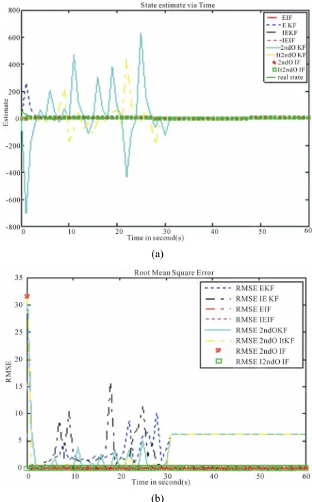
On Figures1(a) and (b), one can observe easily that in the case of high noise level, the information filters are more efficient and more accurate than the classic ap-proximated nonlinear filters based on Kalman filter. At the opposite, on Figures 2(a) and (b) when the noises are low level, we can apply more EKF, IEKF, EIF, and IEIF than the 2nd_{order information filters.}

All the difference between these filters can be seen between 0 and 30 because of the nonlinear measurement equation in this interval of time.

5.2. Consider the Following Set of Equations Such as This Illustrative Example









1

1 2

1

0.5 25 cos 1.2 1

1 k

k k

k

x

1 k

x x

x

 



    

 k v (53)

2

20

k k

x

y  w_k (54)

2nd_{case: (High noise level);}

k = 100; x(1) = 50; y(1) =

100; xr(1) = x(1); yr(1) = y(1); Q(1) = 100; R(1) = 10;

Xest(1) = 0.0.x(1); P(1) = 100; Iterations number: imax = 1000. b− k = 100; x(1) = 50; y(1) = 100; xr(1) = x(1);

(a)

(b)

Figure 1. (a) State, (b) MSE, illustration for the first system with high noise level.

yr(1) = y(1); Q(1) = 100; R(1) = 10; Xest(1) = 0.0.x(1); P(1) = 100; Iterations number: imax=1000.

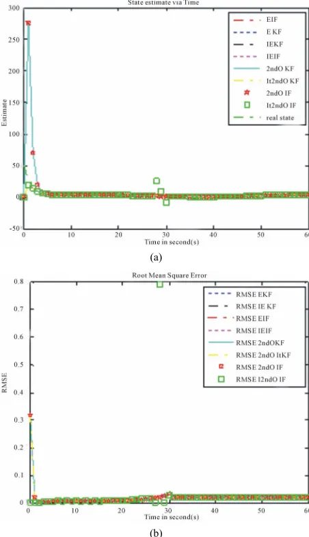
On Figure3, it is easy to observe again that in the case of high noise level, the information filters are more effi-cient and more accurate than the classic approximated nonlinear filters based on Kalman filter.

On Figures4(a) and (b), when the noises are low level, we can apply more nonlinear approximated filters based on Kalman filter than the information filters. One of the most known applications in aerospace and navigation problems are connected with integrated navigations systems and data fusion. This combines between different output of several sensors in order to estimate one or more state variables according to state space model including process and measurement stochastic differential equations.

6. Conclusion

[image:7.595.308.536.84.450.2]

(8)

(a)

(b)

[image:8.595.309.534.82.487.2]

Figure 2. (a) State illustration for the first system with low noise level; (b) MSE, illustration for the first system with Low noise level.

Figure 3. MSE, illustration for the first system with high noise level.

(a)

(b)

Figure 4. (a) State illustration for the first system with low noise level; (b) RMSE illustration for the first system with low noise level.

[image:8.595.58.284.86.478.2] [image:8.595.57.286.534.708.2]

(9)

to high nonlinearity both in system and measurement equations using new formulations of iterative extended Kalman filter, 2nd_{order information filter and 2}nd_order iterative information filter. Finally, original formulations based on sigma point Kalman filters and divided differ-ence information filters are considered to be completed in the near future. It is expected in the future to apply these information filters to integrated navigation system based on combination between GNSS (GPS/GLONASS) and Inertial navigation system (INS) using nonlinear measurement equations in order to compare and confirm that really the new formulations give more accuracy in state estimation’s problems such as started in [29,30] and improved by the novel formulation proposed in this work. Finally, original formulations based on sigma point Kal-man filters and divided difference information filters are considered to be completed in the near future, with addi-tional ways of research on adaptive and robust formula-tions of information filters in very aggressive noise en-vironment.

REFERENCES

[1] R. E. Kalman and R. S. Bucy “A New Approach to Lin- ear Filtering and Prediction Problems,” Journal of Basic Engineering, Vol. 82, No. 1, 1960, pp. 35-45.

http://dx.doi.org/10.1115/1.3662552

[2] R. E. Kalman and R. S. Bucy, “New Results in Linear Filtering and Prediction Theory,” Journal of Basic Engi- neering, Vol. 83, No. 1, 1961, pp. 95-108.

http://dx.doi.org/10.1115/1.3658902

[3] J. Kim, “Autonomous Navigation for Airborne Applica- tions,” Department of Aerospace, Mechanical and Mecha- tronic Engineering, The University of Sydney, Sydney, 2004.

[4] A. V. Nebylov, “Ensuring Control Accuracy,” Springer Verlag, Heidelberg, 2004. 244 p.

http://dx.doi.org/10.1007/b97716

[5] T. Lefebvre, et al. “Kalman Filters for Nonlinear Sys-

tems,” Nonlinear Kalman Filtering, Vol. 19, 2005, pp.

51-76.

[6] S. Thrun, D. Koller, Z. Ghahramani, H. Durrant-Whyte and Y. Ng Andrew, “Simultaneous Mapping and Local- ization with Sparse Extended Information Filters: Theory and Initial Results,” University of Sydney, Sydney, 2002. [7] Y. Liu and S. Thrun, “Results for Outdoor-SLAM Using

Sparse Extended Information Filters,” Proceedings of ICRA, 2003.

[8] M. Simandl, “Lectures Notes on State Estimation of Non- Linear Non-Gaussian Stochastic Systems,” Department of Cybernetics, Faculty of Applied Sciences, University of West Bohemia, Pilsen, 2006.

[9] A. Mutambara, “Decentralised Estimation and Control for Multisensor Systems,” CRC Press, LLC, Boca Raton, 1998.

[10] J. Manyika and H. Durrant-Whyte, “Data Fusion and Sen-

sor Management: A Decentralized Information-Theoretic Approach,” Prentice Hall, Upper Saddle River, 1994. [11] A. Gasparri, F. Pascucci and G. Ulivi, “A Distributed

Extended Information Filter for Self-Localization in Sen- sor Networks,” Personal, Indoor and Mobile Radio Com-

munications, 2008.

[12] M. Walter, F. Hover and J. Leonard, “SLAM for Ship Hull Inspection Using Exactly Sparse Extended Informa- tion Filters,” Massachusetts Institute of Technology, 2008. [13] G. Borisov, A. S. Ermilov, T. V. Ermilova and V. M. Suk-

hanov, “Control of the Angular Motion of a Semiactive Bundle of Bodies Relying on the Estimates of Non- measurable Coordinated Obtained by Kalman Filtration Methods,” Institute of Control Sciences, Russian Acad- emy of Sciences, Moscow, 2004.

[14] N. V. Medvedeva and G. A. Timofeeva, “Comparison of Linear and Nonlinear Methods of Confidence Estimation for Statistically Uncertain Systems,” Ural State Academy of Railway Transport, Yekaterinburg, 2006.

[15] H. Benzerrouk and A. Nebylov, “Robust Integated Navi- gation System Based on Joint Application of Linear and Non-Linear Filters,” IEEE Aerospace Conference, Big

Sky, 2011.

[16] H. Benzerrouk and A. Nebylov, “Experimental Naviga- tion System Based on Robust Adaptive Linear and Non- Linear Filters,” 19th International Integrated Navigation System Conference, Elektropribor-Saint Petersburg, 2011.

[17] H. Benzerrouk and A. Nebylov, “Robust Non-Linear Fil- tering Applied to Integrated Navigation System INS/ GNSS under Non-Gaussian Noise Effect, Embedded Gui- dance, Navigation and Control in Aerospace (EGNCA),” 2012.

[18] T. Vercauteren and X. Wang, “Decentralized Sigma-Point Information Filters for Target Tracking in Collaborative Sensor Networks,” IEEE Transactions on Signal Proc- essing, 2005. http://dx.doi.org/10.1109/TSP.2005.851106

[19] G. J. Bierman, “Square-Root Information Filtering and Smoothing for Precision Orbit Determination,” Factor- ized Estimation Applications, Inc., Canoga Park, 1980. [20] M. V. Kulikova and I. V. Semoushin, “Score Evaluation

within the Extended Square-Root Information Filter,” In: V. N. Alexandrov, et al., Eds., Springer-Verlag, Berlin,

2006, pp. 473-481.

[21] G. J. Bierman, “The Treatment of Bias in the Square-Root Information Filter/Smoother,” Journal of Optimization

Theory and Applications, Vol. 16, No. 1-2, 1975, pp. 165-

178. http://dx.doi.org/10.1007/BF00935630

[22] C. Lanquillon, “Evaluating Performance Indicators for Adaptive Information Filtering,” Daimler Chrysler Re- search and Technology, Germany.

[23] V. Yu. Tertychnyi-Dauri, “Adaptive Optimal Nonlinear Filtering and Some Adjacent Questions,” State Institute of Fine Mechanics and Optics, St. Petersburg, 2000. [24] O. M. Kurkin, “Guaranteed Estimation Algorithms for

Prediction and Interpolation of Random Processes,” Sci- entic Research Institute of Radio Engineering, Moscow, 1999.

(10)

erations Using Ultrafilters of Measurable Spaces,” Insti-tute of Mathematics and Mechanics, Ural Branch, Rus-sian Academy of Sciences, Yekaterinburg, 2006. [26] A. V. Borisov, “Backward Representation of Markov

Jump Processes and Related Problems. II. Optimal Non- linear Estimation,” Institute of Informatics Problems, Russian Academy of Sciences, Moscow, 2006.

[27] A. A. Pervozvansky, “Learning Control and Its Applica- tions. Part 1: Elements of General Theory,” Avtomatika i Telemekhanika, No.11, 1995.

[28] A. A. Pervozvansky, “Learning Control and Its Applica- tions. Part 2: Frobenious Systems and Learning Control for Robot Manipulators,” Avtomatika i Telemekhanika,

No.12, 1995.

[29] V. I. Kulakova and A. V. Nebylov, “Guaranteed Estima- tion of Signals with Bounded Variances of Derivatives,”

Automation and Remote Control, Vol. 69, No. 1, 2008, pp. 76-88. http://dx.doi.org/10.1134/S0005117908010086 [30] Maybeck. “Stochastic Models, Estimations and Control,”