Worker Flows and Firm Dynamics in a Labour Market Model

Munich Personal RePEc Archive

Worker Flows and Firm Dynamics in a

Labour Market Model

Corseuil, Carlos H. L.

July 2009

WORKER FLOWS AND FIRM DYNAMICS

IN A LABOR MARKET MODEL

∗

CARLOS HENRIQUE L. CORSEUIL

Abstract

In this paper we build an integrated framework of the labor market in which worker replacement, job creation and job destruction are decided si-multaneously at the firm level, providing a rigorous instrument for the analy-sis of worker flows. The main features of the model are uncertainty related to worker×firm match quality and search frictions. Worker flow components are decided as firms learn about the quality of their matches. A negative cor-relation between replacement and job creation arises from this mechanism. The model also provides several implications for firm dynamics, which are all confirmed by related empirical papers.

∗_{This material is based on the first chapter of my PhD dissertation developed at}

1

Recent literature on employment dynamics established two empirical regular-ities. The first is the large heterogeneity in employment growth even across similar firms. Davis and Haltiwanger (1999) surveyed several papers on this topic and showed that a significant share of the total variance in employment growth is due to the within group component.1 _{The second fact is that job}

flows and worker replacement occur simultaneously at the firm level, both with significant magnitudes. For instance, Davis and Haltiwanger (1999)2

re-port job flow rates between 15% and 24%, which represent between 41% and 56% of total worker flow rates for annual data of three developed countries.3

The main goal of the present paper is to elaborate a theoretical frame-work that encompasses both of these facts, providing a rigorous instrument for the analysis of worker flows. The framework developed in this paper also has other interesting worker flows predictions that can be used to assess how close the theory matches reality. The model suggests that job creation and replacement should be negatively related to each other, which finds empir-ical support in a companion paper, Corseuil (2009). It also suggests that replacement is negatively related to both wage level and wage growth.

It turns out that the way we model the labor market also generates impli-cations for firm dynamics, even employing the simplest representation of the product market. We offer the following predictions, all confirmed by results

1_{At least 80% according to table 5 in Davis and Haltiwanger (1999) which reports}

results for 13 countries.

2_{See table 9 in their paper.}

3_{See similar numbers in Hamermesh et al. (1996), Davis and Haltiwanger (1998), Albaek}

on firm dynamics surveyed in Sutton (1997); Caves (1998); and Bartelsman and Doms (2000):

- Homogeneous firms (in terms of observable characteristics such as in-dustry, size and age) attain distinct performance levels measured either as productivity at the end of the first period or job creation in the sec-ond period.

- The higher a firm’s initial productivity level, the higher its employment growth.

- Job creation for surviving firms in the second period is negatively cor-related with labor force size at the end of the first period.

- The correlation between job creation and initial size mentioned above tends not to be valid for the largest firms.

- This relationship approaches Gibrat’s Law if we consider the overall population of firms.

- Firms that in the first period are relatively more productive tend to keep this position in the second period.

- Smaller firms have lower probability of surviving than larger firms.

- The variance of employment growth is larger for smaller firms than for larger firms.

quality is assumed to be a non-observable variable, a priori, but eventually will be learned by the firm, which might then seek to improve the overall match composition by trying to form new high quality matches either as part of a worker replacement or a job creation process. We develop a par-ticular formulation for a turnover model which adds search friction to the uncertainty faced by firms concerning the quality of matches. Such complex hiring decisions are mainly responsible for broadening the scope of relevant facts beyond worker flows to firm dynamics.

Most predictions in our paper on firm dynamics are shared with other papers such as Ericson and Pakes (1995); and Klette and Kortum (2004). However, the present paper does not rely on modeling a complex production process with strategic investment decisions taking place, as is the case in those papers. They address investment decisions on R&D or quality improvement, which is more suitable for a high-tech environment. Alternatively, the scope of our model encompasses any firm, from those with the most primitive to those with the most complex production process. To the best of our knowledge, no similar framework is available in the literature. The originality of the model also applies to the worker flow facts encompassed among it’s predictions.

market and implications beyond employment dynamics towards firm dynam-ics is also addressed by Morita (2008). However, his focus is on training decisions as opposed to hiring decisions.

The remainder of this paper is outlined as follows:

We start with a simpler version of the model, which is the object of the next two sections. In section 2 we introduce a simpler version of the model set-up, where jobs are destroyed exogenously, firms set wages, and are allowed to hire at most one worker per period. The solution for this simpler version of the model is derived in section 3. After getting used to the notation and mechanics of the model, we relax the restriction on hiring in section 4. Sections 5 and 6 are devoted to even more general versions of the model where firms bargain wages with workers and jobs are destroyed endogenously. In each of these sections, we discuss how abolishing the restrictive assumptions enlarges the set of model predictions. The final section summarizes the main contributions.

2

2.1

Timing and Information

• Timing

• Match quality

There are two types of worker × firm matches: high quality (+) and low quality (-). They are defined according to the productivity levels, which are 1 and θ respectively.

• Learning

Any new worker × firm combination has,a priori, the probability s of attaining the higher level of productivity.

The true value for the quality of the match is revealed to the current employer at the end of the first period.

2.2

Labor Supply

• Worker population

Worker population is fixed and denoted by L.

• Search activity

Only unemployed workers search for jobs (no on-the-job searches oc-cur).

• Worker decision process

2.3

Labor Demand

• Size limitation

Firms can post at most one vacancy per period, so the maximum em-ployment level is one worker in the first period, and two workers in the second period.

• Firm’s population

Any firm can enter the market in either time period, as long a start-up lump sum cost ν is paid.

• Job destruction

Throughout t1, firms may be hit, with exogenous probability (η), by a

negative productivity shock, forcing them to leave the market at the end of this period.

• Production technology

All firms produce the same good using the same technology, based solely on the employment level of each type of match.4

f(ℓ+t , ℓ−t) = ℓ+t +θ·ℓ−t.

• Product market

Firms are price takers and goods are sold at a fixed price (p).

4_{The following properties for technology apply: i)constant marginal productivity for}

2.4

Match Technology

• Firm’s search activity and wage setting

Firms post vacancies and set wages on the spot market.

• Match probability

An aggregate matching function m(Ub

t, Vt) with constant returns to

scale is the key determinant of the probability of a firm filling a vacancy, which is represented byM(Ub

t, Vt)/Vt=m(Utb/Vt) = m(γt). The inputs

correspond to the total number of job-seeking workers at the beginning of each period (Ub

t) and the aggregate number of vacancies (Vt). The

ratio Ub

t/Vt hereafter is denoted by γt.

• Vacancy cost in the replacement process

A search component of vacancy cost (crep_{) is paid when vacancies are}

posted. This is the only cost paid by the firm when the vacancy is caused by a replacement process.

• Vacancy costs for new jobs

Vacancies caused by the creation of new job positions incur a higher cost (cjc_{) due to an incremental component (c) as described by the}

equation below:

cjc _=crep _+c.

• No vacancy storage

If a vacancy is not filled in the first period, the firm has to pay the associated cost if it decides to post the vacancy again in the second period.

2.5

Critical Comments on Selected Assumptions

Most of the assumptions listed above are used frequently in search models of the labor market. What follows is a brief overview of some of the present paper’s key assumptions about which there is no consensus in the literature. The assumption of match-specific productivity levels is present in Jo-vanovic (1979) and other articles that use his framework to address worker turnover. It contrasts with the assumption on workers’ intrinsic productivity used by Gibbons and Katz (1991) among others. Both share the successful prediction of a negative hazard rate, but they generate different predictions concerning welfare loss of displaced workers. Welfare loss of displaced work-ers due to advwork-erse selection arises only in an environment where productivity is intrinsic to the worker. Empirical papers testing this prediction are not conclusive. While the results in Gibbons and Katz (1991) favor predictions related to workers’ intrinsic productivity, those in Grund (1999); and Song (2007) reject them.

Second, this unit is fully depreciated if not used, and has no depreciation at all if it is used. Alternatively, we can define this extra cost as a maintenance cost for the capital while it is not in use.

Finally, the assumptions on exogenous job destruction, wage setting and size limitation are not discussed here because each of them will be the focus of specific sections of this paper devoted to generalizations of the framework that cames from relaxing those assumptions.

3

3.1

Labor Demand Policy

For the sake of simplifying the exposition of the solution, we begin by dis-cussing labor demand assuming that firms have enough bargaining power to extract all the rent from their workers, setting wages at the same value of what workers gain from unemployment (w = b). Later in this section, we show that this can result from the combination of no on-the-job searches and the productivity level being specific to the match.

in detail according to the type of match formed in the first period.

3.1.1 Incumbent firms with a high quality match

We show in this section that a firm which learns it holds a high quality match will prefer to create a new job position with the single vacancy rather than to replace its worker hired in the first period. The expected profit related to the latter choice (r) can be written as:

Eξ2Eµ2[π2(r |ξ1 = 1)] ={p·[s+θ·(1−s)]−b} ·m(γ2)−c

rep_,

where the first term corresponds to the profit component related to the pro-duction from a match with the expected quality value, taking into account the chance that no match can be formed. The last component is the hiring cost that needs to be paid anyway. If the firm decides to choose the job creation alternative (jc), the analogous equation is the following:

Eξ2Eµ2[π2(jc|ξ1 = 1)] ={p·[s+θ·(1−s)]−b} ·m(γ2)−c

jc

+ (p−b).

p−b > c.

But it is easy to see that the condition does hold since:

p−b >{p·[s+θ·(1−s)]−b} ·m(γ2) =cjc > c,

where the equality above comes from the zero profit condition for start-ups associated with the free entry assumption.5

3.1.2 Incumbent firms with a low quality match

The expected profits for a firm that learns it holds a low quality match will be the following in case of deciding in favor of replacement or job creation, respectively:

Eξ2Eµ2[π2(r|ξ1 =θ)] ={p·[s+θ·(1−s)]−b} ·m(γ2)−c

rep

;

and

Eξ2Eµ2[π2(jc|ξ1 =θ)] = {p·[s+θ·(1−s)]−b} ·m(γ2)−c

jc

+p·θ−b.

The optimal choice now depends on the comparison betweenp·θ−b and

c. We will focus on the more interesting case where:

5

0< p·θ−b < c

In this case, the optimal choice is to fire the worker and post a vacancy to replace him. The condition above seems reasonable, since it says that the rent extracted from the low quality match is positive, but not too large so that keeping the worker is not the best alternative.

3.2

Model Overview and Micro Implications

The labor market represented in our model evolves in the following way. Initially, firms post a vacancy with the corresponding wage. The match quality will vary among firms which succeed in hiring a worker. Firms may then decide to open a new vacancy either to replace the incumbent employee or to create a new position. Displaced workers will enter the job seekers’ pool together with unemployed workers and those coming from firms that have left the market.

It turns out that firms’ decisions on replacement and job creation de-pend on the quality of their matches, where low quality matches lead to replacement and high quality matches to job creation. These heterogeneous decisions lead to the following implications related to the dynamics on size and productivity, which constitute established facts in the empirical litera-ture where these issues are analyzed:6

- Firms whose observable characteristics are homogeneous (industry, size

6_{See for instance Bartelsman and Doms (2000); and Davis and Haltiwanger (1999) who}

and age) attain distinct performance levels measured either as produc-tivity at the end of the first period or job creation in the second period; and

- The higher a firm’s initial productivity level, the higher its employment growth.

A new finding of the model is the negative correlation between the number of workers replaced and the number of jobs created in the second period. However, the limit of only one vacancy per period imposes this negative correlation, since firms are forced to choose only one of these actions. Our goal in the next section is to build a theoretical framework where firms may create new job positions and replace workers simultaneously. In addition, we show that the negative correlation between these variables still holds when we allow firms to choose freely the number of vacancies posted in each period. Moreover, this less restrictive environment also will provide richer implications concerning firm dynamics. Before moving to the next section we dedicate the remainder of this section to discussing two issues that were previously unaddressed: wage determination and model closure.

3.3

Wage and Labor Supply Determination

3.3.1 First period

Firms move first, offering wages that maximize their expected profit condi-tioned on their beliefs about workers’ acceptance policy. Equilibrium occurs when the workers’ acceptance policy for the observed wage offer profile cor-responds to the firms’ beliefs.

In equilibrium, firms will offer constant and homogeneous wages equiva-lent to the unemployment benefit (wt=b) and any unemployed worker will

accept such an offer if (s)he gets one.

It is easy to see that this is a Nash equilibrium. Given search frictions, workers would accept any wage offer greater than or equal to b. Conditioned on this acceptance policy, firms maximize their profits by offering b.

3.3.2 Second period

In the second period firms are involved in two games.

The first, played with workers who were unemployed in the first period, is described in the same way as in the first period. In this game it is easy to see that the same results apply.

The other game is played with incumbent workers who have just revealed their productivity levels to the current employer. The existence of two types of matches is a relevant departure point from the usual assumptions present in search models.

in the second period and also the same one that prevailed in the first period.7

Therefore, this game is equivalent to the previous one and, once more, the equilibrium is w=b.

One can see this solution as a particular case of a wage bargain framework where the firms extract all the rent. Cooper et al. (2007), for example, formulate the wage setting process this way.

3.4

Model Closure

As mentioned earlier, the zero profit condition for start-ups related to the entry cost assumption imposes the following restriction on parameter values in the second period:

{p·[s+θ·(1−s)]−b} ·m(γ2) = cjc+ν.

From this relationship comes the solution for the probability of filling a vacancy, m(γ2). The analogous zero profit condition for start-ups in the first

period is a bit more cumbersome, since it also addresses the present value of the expected profit in the second period, as shown below:

m(γ1)·{s·p·(1−θ)+(p·θ−b)−

cjc

m(γ1)

− ν m(γ1)

+ρ′·s·m(γ2)·(p−b)+ρ′·(1−s)·c}= 0.

However it can be seen that the expression above is just a function of

m(γ1) and m(γ2). We can then derive the value of the first parameter,

7_{As in the first period the job seeker pool is considered by the firms as a homogeneous}

provided that we previously have solved the value for the second parameter. The fact that we have assumed that m(γt) is a monotonic transformation

of γt means that we can recover the values of γ1 and γ2. These parameters

are the ratio between the number of job seeking workers and the number of vacancies at the beginning of the respective periods. In the first period, all workers are job seekers, which sets Ub

1 =L.

The last step for the closure of the model in the first period is to obtain the value of V1, the aggregate vacancy level in the first period, from γ1 and

Ub

1 = L. Note that in this version of the model, V1 also corresponds to the

number of firms posting vacancies at the beginning of the first period.8 _The

aggregate vacancy level in the second period, V2, can be obtained in the

same way. However the number of job seeking workers in the beginning of the second period, Ub

2, does not corresponds to L anymore. In the second

period we have to address the inflows and outflows from unemployment as shown below:

Ub

2 =U1+JD+R = (L−M1) +η·M1+ (1−η)·(1−s)·M1,

whereM1 stands for the number of matches formed in the first period, which

corresponds to m(γ1)·V1. It is easy too see that U2b depends on quantities

that have their values already determined above. Then we can plug Ub

2 into

m(γ2) to get the value of V2. The number of vacancies posted in the second

period by incumbent firms is (1−η)·m(γ1)·V1, while the remaining vacancies

8_{This is not the same as the number of operating firms in the first period due to search}

will be posted by start-ups.

4

The aim of this section is to generalize the theoretical framework to allow firms to choose freely the number of vacancies posted. Obviously this proce-dure will make the analysis of the labor demand policy more cumbersome. On the other hand, wage and labor supply determinations remain unchanged. For this version of the model, we still rely on most of the assumptions stated previously. Those that need to be amended are restated below.

4.1

Assumptions

• Size limitation II

Firms can hire any number of workers in either time period.

• Match probability II

The probability of a firm fillingℓtof itsvtopen vacancies is independent

of the number of posted vacancies, and given by m(γt) as before.

• Vacancy cost in the replacement process II

The search component of vacancy cost is convex. For the sake of conve-nience, we will use the following quadratic parametrization, crep_(v

t) =

a·v2_{, witha >0 defining the curvature of this cost function.}

A vacancy due to the creation of a new job position has an extra linear component to be paid. The following equation summarizes the relation between the two cost components: cjc_(v

t) = crep(vt) +c·v, withc >0.

The assumption of convex vacancy cost deserves comment. It is shared with Bertola and Caballero (1994); Bertola and Garibaldi (2001); Garibaldi (2006); and Garibaldi and Moen (2008). This is a critical assumption for our results on firm dynamics. Although it contrasts with the standard assump-tion of linear costs present in most unemployment matching models, it is an assumption critical to our results on firm dynamics. Not only do Garibaldi and Moen (2008) provide theoretical justification for this assumption, there also is empirical evidence supporting the convex shape. Yashiv (2000) points out that a structural estimation of the standard matching model performs better with convex than with linear specification for the hiring cost. Cooper et al. (2004) claim that a quadratic shape with a disruption component fits the data better than the alternatives considered, including the linear case.9

An important difference to be noted in these two papers is that the first uses gross hirings and separations as a measure of labor adjustment while the second uses net employment growth. Hence, the intercept in Cooper et al. (2004) may be related to the fact that firms may pay adjustment costs even when they do not grow, as long as they hire workers to replace others.

9_{Cooper et al. (2004) stress that the quadratic component is close to zero, but its}

4.2

Labor Demand

The problem of choosing the vacancy level raises the level of complexity of labor demand policy in both periods. In the second period, firms now have to address two choices, which are: 1) how much to spend on improving the quality of the matches; and 2) how much to spend on increasing the number of jobs. The first choice consists in choosing the number of workers to be replaced, while the second consists of choosing the number of vacancies allocated to job creation. In the first period, firms now face a dynamic environment, in that their first period decisions on vacancy level will affect their available choices in the second period. Therefore, the solution to the firm problem will be stated below in the form of backward induction.

4.2.1 Start-up in the second period

Employment policy for start-up firms in the second period is the simplest case to be considered since the choice set for these firms is not influenced by past decisions. In this case, firms just choose the number of vacancies to post (v2). The profit of a firm which hiresℓ+2 and ℓ−2 when postingv2 vacancies is

represented by the following equation:

π2(v2 |ℓ+2, ℓ−2) =p·(ℓ+2 +θ·ℓ−2)−b·ℓ2−cjc(v2)−ν.

Howeverℓ+₂ and ℓ−₂ are not under the firm’s control. They are defined by the success rate in filling vacancies (µ2) and the proportion of high quality

matches (ξ2). These random variables have expected values s and m(γ2)

expected profit concerning these two variables, as described by:

Eξ2Eµ2[π2(v2)] ={p·[s+θ·(1−s)]−b} ·m(γ2)·v2−a·v 2

2−c·v2−ν.

The convex shape of the cost function guarantees that there is only one maximum associated with an optimal vacancy level, to which we will refer as vst

2 . It is easy to see that

vst

2 =

{p·[s+θ·(1−s)]−b} ·m(γ2)−c

2·a .

The only endogenous parameter on the right side of this equation ism(γ2),

which is determined by the free entry condition.10

4.2.2 Incumbent firms in the second period

Employment policy in the second period is more complex for incumbent firms. Between the first and second periods, they decide on the number of workers to be replaced (r) and the number of new job positions to be created (jc), having been informed about first period labor force size (ℓ1) and the quality

of the matches (ξ1). We can write in the following way the second period

profit of a firm which hires ℓ+₂ and ℓ−₂, when posting r vacancies devoted to replace workers in low quality matches and jc vacancies to create new job positions:

10_{There is a unique value for this parameter that is associated with zero profit for}

π2(r, jc|ℓ+2, ℓ−2, ℓ+1, ℓ−1) = p·(ℓ+2 +θ·ℓ−2)−b·ℓ2−

p·(ℓ+₁ +θ·ℓ−₁)−b·ℓ1−[(p·θ−b)·r] + [cjc(jc+r)−c·r].

The terms on the right side in the first row refer to the profit compo-nent derived from the production associated to workers hired in the second period. The second row starts with the profit component derived from the production associated to workers hired in the first period, discounting the related production of those workers replaced in the second period. The last term corresponds to vacancy costs taking into account that some of these may be allocated to replacement while the remaining to job creation. All the other terms have straightforward interpretations.

The equation above uses the following facts:

- Any displacement of workers not related to a replacement process is not considered since both types of matches are profitable; 11 _and

- Firms will never replace any worker in a high quality match, since no new worker can be more profitable.

As mentioned earlier, the objective function to be maximized by the firms is the expected profit regarding the random variables ξ2 and µ2, which can

be described as below:12

11_{This comes from the fact that}

p·θ > b.

12_{We use the facts that}

Eξ2Eµ2[π2(r, jc |ξ1, ℓ1)] ={p·[s+θ·(1−s)]−b} ·m(γ2)·(jc+r)−

cjc(jc+r) +p·[ξ1 ·ℓ1+θ·(1−ξ1)·ℓ1]−b·ℓ1+ [c−(p·θ−b)]·r.

Note that the number of replacements should be no greater than the number of low quality matches, therefore, the incumbent firms’ problem can be stated as:

max

r,jc Eξ2Eµ2[π2(r, jc|ξ1, ℓ1)] (1)

s.t. r ≤ℓ−₁.

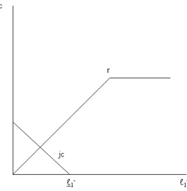
The application of the Kuhn-Tucker conditions for this problem is shown in Appendix A. The optimal number of worker replacements and job creation shown in figure 1 are defined as:

r∗ =

  

 

ℓ−₁, ℓ−₁ < ℓ−

ℓ−_{, ℓ}−

1 ≥ℓ−

(2)

and

jc∗ =

  

 

ℓ−_−ℓ−

1, ℓ−1 < ℓ−

0, ℓ−₁ ≥ℓ−_;

(3)

ℓ− = z2 2·a

and

ℓ−₌ z2+k

2·a ;

with z2 and k defined as:

z2 ={p·[s+θ·(1−s)]−b} ·m(γ2)−c

and

k = [c−(p·θ−b)].

Note that in the previous section we have mentioned that we would con-sider the case where (p·θ−b)< c, which in turn guarantees that ℓ− _{< ℓ}−_.

There are two important features to be stressed in these expressions. First, the solution for the choice variables is guided by the number of low quality matches. So, the heterogeneity of the latter variable across firms im-plies heterogeneous choices of replacement and job creation as well. Second, when the levels of job creation and replacement are compared across firms, it turns out that they are negatively related to each other at the ratio of one-to-one for some region below a threshold level of ℓ−1 and they then become

unrelated to each other for higher values of ℓ−

4.2.3 Start-ups in the first period

We are now ready to tackle the problem that firms face in the first period using the results derived above. It will be useful to denote the value function of the expected profit at the beginning of the second period, conditioned on realizations of ξ1 and ℓ1 as:

Eξ2Eµ2[π2(r

∗_{, jc}∗_{, ξ}

1, ℓ1)]

This represents the expected profit for a firm that behaves optimally in the second period, having hired ℓ1 workers in the first period, among which

the share of good matches turns out to be ξ1.

Note that the values of ξ1 and ℓ1 are not known at the beginning of the

first period. At this time firms may infer these values conditioned on the vacancy level chosen (v1).

Denoting as ρ′ _{the composed discount rate that takes into account the}

survival probability (ρ′ _{=ρ·(1−η)), the first period decision can be}

repre-sented as

max

v1

E1[π(v1)] = max

v1

{E1[π1(v1)] +ρ′·E1[π2∗ |v1]}. (4)

EξEµ1[π1(v1)] =

{p1·[s+θ·(1−s)]−b} ·m(γ1)·v1−cjc(v1)−ν =

(z1−c)·v1−a·(v1)2 −ν,

where

z1 ={p1·[s+θ·(1−s)]−b} ·m(γ1).

As shown in Appendix B, E1[π2∗ |v1] is defined as

E1[π2∗ |v1] =z1·v1−ν+

                                          

(z2+k)·ℓ−−a·(ℓ−)2,

v1 > v1

(z2+k)·(1−s)·m(γ1)·v1−a·E1[(ℓ−1)2 |v1],

v1 < v1 < v1

z2·ℓ−+k·(1−s)·m(γ1)·v1−a·(ℓ−)2,

v1 < v1.

E1[π1(v1) +ρ′·E1[π∗2 |v1]] = [1 +ρ′]·z1·v1 −a·(v1)2−c·v1+

(5)

ρ′_·                       

(z2+k)·ℓ−−a·(ℓ−)2, v1 > v1

−a·E1[(ℓ−1)2 |v1] + (z2+k)·(1−s)·m(γ1)·v1, v1 < v1 < v1

z2 ·ℓ−−a·(ℓ−)2+k·(1−s)·m(γ1)·v1, v1 < v1.

The equation above combines quadratic and linear terms in v1. This

guarantees that local maxima are well defined. Nevertheless, the uniqueness of a global maximum depends on the values imposed for the parameters of the model. Figure 2 aids in understanding the above expression. In Appendix C we show that global maximum uniqueness is attained for a sufficiently large

s.

Note that even when firms post the same number of vacancies, they will differ in two aspects at the end of the first period: i) labor force size and ii) la-bor force composition. These are consequences of the stochastic environment in which hiring occurs.13

13_{Another dimension in which firms will differ at this stage is productivity as an obvious}

4.3

Updates in Model Overview and Micro Predictions

One of the main goals of the model developed above was to reproduce the fact that some firms replace workers and create new jobs simultaneously. The mechanism of firm dynamics that comes from the enriched set of assumptions used in this version of the model generates other predictions which can be used to check the pertinence of the model.

The dynamic mechanism of this version of the model is very similar to the one used for the simpler version described earlier. The difference is that the driving force here is the number of low quality matches formed in the first period. Those firms with low levels of ℓ− _{create jobs and replace fewer}

workers. Those firms with high levels of ℓ− _{focus their hiring efforts on the}

replacement process and create relatively fewer jobs or even do not create any jobs at all.

Bearing in mind that µt and ξt are independent, the initial level of low

quality matches is positively correlated with the initial labor force size. As a consequence of this result we predict that:

- Job creation in the second period is negatively correlated to labor force size at the end of the first period.

This corresponds to the correlation between size and growth for surviving firms pointed by Sutton (1997). The author writes: “...the proportional rate of growth of a firm (or plant) conditional on survival is decreasing in size.”14

Note that in our model there is a threshold initial level ofℓ− _{above which}

the vacancy level does not depend on this variable anymore. Therefore we

can add the following remark to the prediction above:

- The relationship between job creation and initial size pointed out before tends not to be valid for the largest firms.

This is precisely how Caves (1998) puts the relationship between employ-ment growth and initial size: “...mean growth rates of firms decrease with their initial sizes among small firms; for initially large firms growth rates and size are unrelated.”15

In terms of productivity, the model predicts that those firms in disadvan-tage (high ℓ−₁) will make more effort to improve the composition concerning match quality. Hence, there is a catch-up process in terms of match quality composition which, in other words, means a catch-up in terms of productiv-ity. It is not difficult to see that the catch-up is limited as described below:

- Firms that in the first period are relatively more productive tend to keep this relative position in the second period.

This prediction finds strong support, this time from Bartelsman and Doms (2000): “...highly productive firms today are more than likely to be highly productive firms tomorrow...”16_.

5

We will show that the problem that firms solve to determine their hiring policy under wage bargaining is extremely similar to the one postulated under

the wage setting environment developed in the previous sections. The set-up is the same as the previous model except for the assumption on wage setting which can now be stated as:

• Firm’s search activity and wage setting II

Firms post vacancies and bargain wages on the spot market, with bar-gaining power 1−β.

5.1

Model Solution: Wage Determination

Based on the last assumption, the wage determination can be easily devel-oped. Bargaining will be conducted conditioned on the information available for match productivity. This information determines the rent to be split between firm and worker according to their respective bargaining power. Therefore we have three possible situations:17

• An ongoing match in the second period revealed to be of high quality, in which case the wage is defined as:

w+=β·p+ (1−β)·b;

• An ongoing match in the second period revealed to be of low quality, in which case the wage is defined as:

w−_{=β·p·θ+ (1−β)·b;}

17_{The derivations of the value for the wage given the value of the match productivity are}

and;

• A newly formed match either in the first or second period in which case the productivity is not known and the expected value iss+ (1−s)·θ. Therefore the wage is:

we =β·p·[s+ (1−s)·θ] + (1−β)·b.

5.2

Model Solution: Labor Demand

5.2.1 Start-up in the second period

As developed in the previous section, start-ups in the second period choose the number of vacancies that maximize their expected profit, which in this case becomes

Eξ2Eµ2[π2(v2)] ={p·[s+θ·(1−s)]−w

e_{} ·m(γ}

2)·v2−a·v22−c·v2−ν.

Using the value derived above for we_{, we have}

Eξ2Eµ2[π2(v2)] = (1−β)· {p·[s+θ·(1−s)]−b} ·m(γ2)·v2−a·v 2

2−c·v2−ν.

It is easy to see that the only difference from the analogous definition in the wage setting version of the model is the pre-multiplication of (1−β) in the first term. This is also the case for the value of vst

as:

vst₂ = (1−β)· {p·[s+θ·(1−s)]−b} ·m(γ2)−c

2·a .

5.2.2 Incumbent firms in the second period

Again, the objective function to be maximized by firms is the expected profit regarding the random variablesξ2 andµ2. Under wage bargaining, it can be

described as:18

Eξ2Eµ2[π2(r, jc|ξ1, ℓ1)] = {p·[s+θ·(1−s)]−w

e_{} ·m(γ}

2)·(jc+r)−

cjc(jc+r) +ℓ1· {(p·ξ1−w+) + [p·θ·(1−ξ1)−w−]}+ [c−(p·θ−w−)]·r.

Using the values derived above for we_{, w}+ _{and w}− _{we have}

Eξ2Eµ2[π2(r, jc|ξ1, ℓ1)] = (1−β)· {p·[s+θ·(1−s)]−b} ·m(γ2)·(jc+r)−

cjc(jc+r) + (1−β)·ℓ1·[(p·ξ1−b) +p·θ·(1−ξ1)−b] + [c−(1−β)·(p·θ−b)]·r.

As in previous sections, the firm labor demand decision can be solved through the following maximization problem:

18_{We use the facts that}

max

r,jc Eξ2Eµ2[π2(r, jc|ξ1, ℓ1)] (6)

s.t. r ≤ℓ−₁.

The only difference from the analogous definition for the expected profit in the wage setting version of the model is the pre-multiplication of (1−β) in some terms. So the solution for this maximization problem will be analogous to the one developed for the wage setting version of the model, where both replacement level and job creation depend on ℓ−₁ and the parameters of the model, as shown in figure 1. The only adaptation necessary for this version of the model is that the expressions for ℓ−1 and ℓ−1 includeβ:

ℓ′− = z

′

2

2·a

and

ℓ′₋

= z

′

2+k

′

2·a

wherez′

2 and k

′

are defined as:

z2′ = (1−β)· {p·[s+θ·(1−s)]−b} ·m(γ2)−c

k′ = [c−(1−β)·(p·θ−b)].

version of the model and the wage setting version depends on a necessary condition being met: that the probability of finding a job (m(_γγ₂2)) is not too high for a job seeking worker at the beginning of the second period.

5.3

Predictions on Wage Dynamics

The introduction of wage variation with the wage bargaining set-up devel-oped above allows us to expand the scope of model predictions on worker flows. It is easy to realize the following relationship between wages and worker flows:

- At the individual level, the probability of remaining employed in the same firm is positively associated with the wage level in the second period and the wage growth between the two periods.

This prediction is confirmed by the findings of Topel and Ward (1992), a widely quoted empirical paper on the determinants of the mobility of (young) workers. As a consequence of this result, we may state that:

- At the firm level, the average wage level in the second period is nega-tively correlated to the replacement level.

6

6.1

Generalizing Incumbent Firms’ Decisions

Until now we have assumed that all firms face a positive probability of leaving the market at the end of the first period due to an exogenous negative shock. Now we want to relax this assumption. We follow standard models of firm dynamics and allow firms to choose, at the end of the first period, whether to continue or stop their operations. In case of giving up, they are compensated with a scratch value (ψ) and their employees will join the group of workers searching for jobs between the end of the first period and the start of the second period. In case of continuing their activities, they choose replacement and job creation levels as described in the last section. The firm decision in the second period can be written then as

max

r,jc,χ χ·Eξ2Eµ2[π2(r, jc|ξ1, ℓ1)] + (1−χ)·ψ (7)

s.t. r ≤ℓ−₁,

whereχ values 1 when the firm decides to continue and 0 otherwise. We can see this problem as adding another layer to the decision process of the firm. After solving for the optimal levels of r and jc based on the expected profit associated with continuing their operations, firms compare this later magnitude with ψ to decide whether to continue or not.

more convenient to write the value function of the second period continuation expected profit as a function of ℓ−₁ and ℓ+₁:

Eξ2Eµ2[π2(r

∗_{, jc}∗_{, ℓ}−

1, ℓ+1)] = p·[ℓ+1θ·ℓ−1]−b·(ℓ+1 +ℓ−1)

(8)                       

z2·ℓ−+k·ℓ−1 −a·(ℓ−)2, ℓ−1 < ℓ−

(z2+k)·ℓ−1 −a·(ℓ−1)2, ℓ− < ℓ−1 < ℓ−

(z2+k)·ℓ−−a·(ℓ−)2, ℓ−1 > ℓ−.

The second step consists of defining the locus of points where

Eξ2Eµ2[π2(jc

∗_{, r∗, ℓ}−

1, ℓ+1)] =ψ.

Figure 3 shows the shape of this locus on the planeℓ−_×ℓ+_{(see the}

deriva-tion of this shape in Appendix E). This line defines a border where points to the lower/left constitute the exit region, while points to the upper/right region constitute the stay region.

6.2

Further Implications on Firm Dynamics

firms.19 _{It should be stressed though that this is not a deterministic}

rela-tionship. For any firm in our “exit” region, but close enough to the border, one can always find another firm of the same size, or even smaller, located in our “stay” region.20 The non-deterministic negative relationship between size and exit probability also features in the main theoretical frameworks of firm dynamics, such as Ericson and Pakes (1995); and Klette and Kortum (2004).

The fact that smaller firms are more inclined to leave the market provides two other implications which are frequently mentioned in the literature of firm dynamics. First, it makes the variance of employment growth larger for this group than for larger firms. Second, the relationship between initial size and employment growth for the overall firm population (including those withdrawing from the market) is closer to Gibralt’s Law, than when we restrict the population to surviving firms.21

7

In this paper we developed a labor market model where several facts on worker flow and firm dynamics were rationalized exclusively through em-ployment decisions made by the firms. The main characteristics of the model were imperfect information about the quality of new matches and search fric-tions. When hiring workers, firms do not know whether there will be enough workers to fill the open vacancies and, once a new worker comes in, they do

19_{A smaller firm tends to be to the left and below a larger firm.} 20_{This is where the inclination lower than one is important.}

21_{Gibrat’s Law says that firms’ employment growth rates are independent of size. Sutton}

not know the productivity level of that worker × firm match.

In developing this model we built an integrated framework of the labor market in which replacement, job creation and job destruction were decided simultaneously at firm level. We have shown that several interesting micro implications come from this framework. These implications are not restricted to matters of worker flows, as they also encompass some facts on firm dy-namics. Moreover, we showed that all the results derived for firm dynamics match empirical evidence documented by the related literature.

It should be stressed that other papers which offer comparable predictions on firm dynamics rely on some sort of investment decision composing a more elaborate production process. In our framework, the driving force for firm dynamics was the same as for worker flows, namely the learning process about match quality.

Desirable extensions of our framework would be an infinite horizon over-lapping generation model to explore the macro implications of the model, and the effects of policy experiments. This framework would be able to pre-dict coherently the effects of such experiments on several dimensions, such as job flows, unemployment flows, unemployment level, firms’ size distribution and firms’ productivity distribution. This provides valuable information for the welfare analysis of alternative policy interventions. For example, altering firing costs, social contributions or minimum wage potentially will affect all the above mentioned dimensions.

Appendices

A

The incumbent firm solves the following problem in the interim between first and second periods:

max

r,jc Eξ2Eµ2[π2(r, jc|ξ1, ℓ1)]

s.t. r ≤ℓ−₁.

Another way of stating this problem, making the argument to be maxi-mized an explicit function of r and jc, is the following:

max

r,jc {z2·(jc+r)−a·(jc+r)

2_+k·r+p·[ξ

1·ℓ1+θ·(1−ξ1)·ℓ1]−b·ℓ1}

s.t. r ≤ℓ−₁

wherez2 and k correspond to:

z2 ={p·[s+θ·(1−s)]−b−c} ·m(γ2)−c

and

k = [c−(p·θ−b)].

three blocks of restrictions that need to be satisfied. The first is related to

jc, the second to r, and the last to the lagrangian multiplierλ:

z2−2·a·(jc+r)≤0

jc≥0

[z2−2·a·(jc+r)]·jc= 0

z2 −2·a·(jc+r) +k−λ≤0

r ≥0

[z2−2·a·(jc+r) +k−λ]·r= 0

ℓ−₁ −r ≥0

λ≥0

(ℓ−₁ −r)·λ= 0

The following combinations of values for r and jc can occur:

• jc > 0 andr =ℓ−₁

z2−2·a·(jc+r) = 0.

Plugging this into the second block we get λ ≥ k, which implies a positive λ. When we take this to the third block, we get r =ℓ−₁. The value of jccan then be written as

jc= z2 2·a −ℓ

−

1.

Finally, in order to have jc > 0, the following condition must be satis-fied:

ℓ−₁ < z2

2·a.

• jc= 0 andr =ℓ−₁ >0

According to the first block of equations above, if jc= 0 then

z2−2·a·r ≤0,

which implies

ℓ−

1 ≥

z2

2·a.

Concerning the restrictions on r, if r >0, the second block implies

On the other hand when we use r=ℓ−₁ in the third block, we get:

λ≥0

Putting these two conditions together we have:

ℓ−₁ ≤ z2+k

2·a .

So the combination of jc= 0 andr=ℓ−₁ >0 occurs when:

z2

2·a ≤ℓ

−

1 ≤

z2+k

2·a .

• jc= 0 andr < ℓ−₁

The relationships between z2 and r derived above from jc = 0 and

r >0 remain valid. We repeat them below for convenience:

z2−2·a·r≤0

z2−2·a·r+k =λ.

However, when we take r < ℓ−₁ to the third block above we get λ = 0. We can use this fact to recover the value of r from the equation above as

which in turn implies that

ℓ−₁ > z2+k

2·a .

B

First, consider the following value function defined according to the optimal labor demand policy in the second period:

π2(ξ1, ℓ1, r∗, jc∗) = p·[ξ1+θ·(1−ξ1)]−b·ℓ1+z2·(jc∗+r∗)−a·(jc∗+r∗)2+k·r∗.

However, we have seen thatr∗ _andjc∗ _{are defined according to ℓ}−

1, which

in turn can be expressed as (1−ξ1)·ℓ1. So, plugging this definition ofℓ−1 into

the solution for replacement and job creation allows us to write the second period profit as

π∗

2(ξ1, ℓ1) ={p·[ξ1+θ·(1−ξ1)]−b} ·ℓ1+

(9)                       

(z2+k)·ℓ−−a·(ℓ−)2, ℓ−1 > ℓ−

(z2+k)·(1−ξ1)·ℓ1−a·[(1−ξ1)·ℓ1]2, ℓ− < ℓ−1 < ℓ−

When firms are in the first period, they will look to the expected value of the second period profit conditioned on the first period vacancy level, which can be defined as below.

E1[π2∗ |v1] =z1·v1+

(10)                                           

(z2 +k)·ℓ−−a·(ℓ−)2,

(1−s)·m(γ1)·v1 > ℓ−

(z2 +k)·(1−s)·m(γ1)·v1−a·E1[(ℓ−1)2 |v1],

ℓ−_{<(1−s)·m(γ}

1)·v1 < ℓ−

z2·ℓ−−a·(ℓ−)2 +k·(1−s)·m(γ1)·v1,

(1−s)·m(γ1)·v1 < ℓ−.

We have used the following facts: µ1⊥ξ1, E[ξ1 | v1] = E[ξ1] = s and

E[ℓ1 |v1] =m(γ1)·v1.

It would be useful to redefine the inequalities above in terms of v1. It is

easy to see that

v1 =

ℓ−

(1−s)·m(γ1)

v1 =

ℓ−

(1−s)·m(γ1)

This completes our derivation for the second component of first period expected profit, which becomes:

E1[π2∗ |v1] =z1·v1+

(11)                                           

(z2 +k)·ℓ−−a·(ℓ−)2,

v1 > v1

(z2 +k)·(1−s)·m(γ1)·v1−a·E1[(ℓ−1)2 |v1],

v1 < v1 < v1

z2·ℓ−−a·(ℓ−)2 +k·(1−s)·m(γ1)·v1,

v1 < v1.

C

1

E1[π1(v1) +ρ′·E1[π∗2 |v1]] = [1 +ρ′]·z1·v1 −a·(v1)2−c·v1+

(12)

ρ′_·                       

(z2+k)·ℓ−−a·(ℓ−)2, v1 > v1

−a·E1[(ℓ−1)2 |v1] + (z2+k)·(1−s)·m(γ1)·v1, v1 < v1 < v1

z2 ·ℓ−−a·(ℓ−)2+k·(1−s)·m(γ1)·v1, v1 < v1.

First, we disaggregate E1[π∗2(v1)] into linear and non-linear components,

denoting them respectively by Rmg(v1) and Cmg(v1). They are illustrated

in figure 2 which shows three different regions (a, b and c) delimited by v1

and v1. Suppose the following restrictions hold:

Rmg−(v1)< Cmg−(v1)

Rmg+(v1)< Cmg+(v1)

Rmg+(v1)< Cmg+(v1)

holds:

π(va∗)> π(v∗b) = π(v1)> π(v1) = π(v∗c).

The first and second restrictions correspond to the ones shown below. The third one is not binding, since its requirement is guaranteed by the first restriction:

2·a·v1 >(1 +ρ′)·z1−c+k·ρ′·(1−s)·m(γ1)

2·a·v1+ρ′ ·a·

∂E1[(ℓ−

1) 2

|v1]

∂v >(1 +ρ

′_)·z

1−c+ (k+z2)·ρ′ ·(1−s)·m(γ1).

Now consider the first inequality above. It can be rewritten as:

z2

(1−s)·m(γ1)

>(1 +ρ′)· (z2+c)·m(γ1) m(γ2)

−c+k·ρ′·(1−s)·m(γ1),

using the definition for v1 and the fact that

z1 =

(z2+c)·m(γ1)

m(γ2)

.

In the remainder of this section we will assume m(γ1) ∼= m(γ2), for the

z2·

[1−(1 +ρ′_{)·(1−s)·m(γ}

1)

(1−s)·m(γ1)

> ρ′_·c+k·ρ′_{·(1−s)·m(γ}

1).

Finally, the fact that ∂z2

∂s > 0 guarantees that the first inequality holds

when we increase s. The second inequality can be written as

z2·

[1−(1 +ρ′_{)·(1−s)·m(γ}

1)

(1−s)·m(γ1)

−ρ′ ·c+k·ρ′·(1−s)·m(γ1)

> z2·ρ′ ·(1−s)·m(γ1)−ρ′ ·a·

∂E1[(ℓ−1)2 |v1]

∂v .

We have just shown that the left hand side (LHS) is greater than zero for a large enough s. The right hand side (RHS) can be restated as:

z2·ρ′·(1−s)·m(γ1)−

z2·ρ′·(1−s)

m(γ1)

− z2 ·ρ

′_·x

m(γ1)·(1−s)

where we have used the result below:

∂E1[(ℓ−1)2 |v1]

∂v = 2·a·v1· {(1−s)2+var(1−s) + [m(γ2)]2+var[m(γ2)]2}

to see that this RHS is negative for any s, which allows us to establish the following relationship:

LHS > 0> RHS

Thus, a big enoughs in an environment where m(γ1) =m(γ2) suffices to

guarantee a unique solution for v∗

1 at a level lower than v1.

D

SO-LUTION OF THE WAGE BARGAINING VERSION OF

THE MODEL

Consider a match that is revealed to be of low quality. At the beginning of the second period, the worker in this match may decide either to quit or to stay. The expected payoffs (EP) related to each of these two decisions, identified by superscripts, are the following:

EPq =q· {p·β·[s+ (1−s)·θ] + (1−β)·b}+ (1−q)·b

and

EPs =p·β·θ+ (1−β)·b,

where q represents the probability of a job seeking worker finding a job at the beginning of the second period, which is given by m_γ(γ2)

2 . Straightforward

f(q)< p·θ−b,

where f(q) abbreviates p·q·θ +p·q·s·(1−θ)−b·q. In what follows we will show that any value for q below a threshold will make such workers prefer to stay, as in the wage setting version of the model. First, note that the condition is attained when q = 0. Hence showing thatf′_{(q) >0 suffices}

to prove our claim. In fact, we have that

f′(q) = p·[s+ (1−s)·θ]−b >0.

Finally, the threshold value for q which makes the worker indifferent be-tween quitting and staying is:

q∗ ₌ p·θ−b

p·[s+ (1−s)·θ]−b.

E

The main component of the exit rule consists of a line on the plane ℓ−₁ × ℓ+₁

which represents the locus of points where

Eξ2Eµ2[π2(jc

∗_{, r∗ |ℓ}−

1, ℓ+1)] =ψ.

The shape of this line is given by the partial derivative ofℓ+

1 with respect

toℓ−₁ keeping constant the value function above. That is, we need to compute:

∂ℓ+₁ ∂ℓ−₁

¯ ¯ ¯ ¯

Eξ2Eµ2[π2(jc∗,r∗|ℓ

−

1,ℓ + 1)]=ψ

Straightforward derivations imply that:

∂ℓ+₁ ∂ℓ−1

¯ ¯ ¯ ¯

Eξ2Eµ2[π2(jc∗,r∗|ℓ−1,ℓ + 1)]=ψ

= 1

p−b

                                          

−[(p·θ−b) +k], ℓ−₁ < ℓ−

2·a·ℓ−₁ ·[(p·θ−b) +k+z2],

ℓ− < ℓ−1 < ℓ−

−(p·θ−b), ℓ−₁ < ℓ−_.

It is easy to see that the the first and last regions have negative and con-stant inclinations. In the intermediary region (ℓ− _{< ℓ}−

1 < ℓ−) the inclination

raises monotonically with the level of ℓ−₁. Plugging into the equation values for ℓ− _{and ℓ}−_{, one can see that the slope in this region varies monotonically}

from the value of the first region to the value of the last region.

References

J. Abowd, P. Corbel, and F. Kramarz. “The entry and exit of workers and the growth of employment: an analysis of French establishments”. Review of Economics and Statistics, 81:170–187, 1999.

K. Albaek and B. Sorensen. “Worker Flow and Job Flow in Danish Manu-facturing, 1980-91”. The Economic Journal, 108:1750–1771, 1998.

E. Bartelsman and M. Doms. “Understanding Productivity: Lessons from Longitudinal Microdata”. Journal of Economic Literature, 38:569–594, 2000.

G. Bertola and R. Caballero. “Cross-sectional efficiency and Labour Hoarding in a Matching Model of Unemployment”. Review of Economic Studies, 61: 435–456, 1994.

G. Bertola and P. Garibaldi. “Wages and the Size of Firms in Dynamic Matching Models”. Review of Economic Dynamics, 4:335–368, 2001.

S. Burgess, J. Lane, and D. Stevens. “Job Flow, Worker Flow and Churning”.

Journal of Labor Economics, 18:473–502, 2000.

S. Burgess and H. Turon. “Worker Flows, Job Flows and Unemployment in a Matching Model”, 2005. Bristol Economics Discussion Papers.

R. Cooper, J. Haltiwanger, and J. Willis. “Dynamics of Labor Demand: Ev-idence from Plant-level Observations and Aggregate Implications”, 2004. NBER working paper 10297.

R. Cooper, J. Haltiwanger, and J. Willis. “Implications of Search Frictions: Matching Aggregate and Establishment-level Observations”, 2007. NBER working paper 13115.

C. H. Corseuil. “Alternative Ways of Measuring and Interpreting Worker Flows”, 2009. mimeo.

S. Davis and J. Haltiwanger. Measuring gross worker and job flows. La-bor Statistics Measurement Issues. NBER, Chicago, 1998. editors Haltin-wanger, Manser and Topel.

S. Davis and J. Haltiwanger. Gross job flows, volume 3B of Handbook of Labor Economics. North Holland, 1999. editors Orley Ashenfelter and David Card.

R. Ericson and A. Pakes. “Markov Perfect Industry Dynamics: A Framework for Empirical Work”. Review of Economic Studies, 62:53–82, 1995.

M. Galizzi and K. Lang. “Relative Wages, Wage Growth, and Quit Behav-ior”. Journal of Labor Economics, 16:367–391, 1998.

P. Garibaldi. “Hiring Freeze and Bankruptcy in Unemployment Dynamic”, 2006. CEPR discussion paper 5835.

R. Gibbons and L. Katz. “Layoffs and Lemons”. Journal of Labor Economic, 9:351–380, 1991.

C. Grund. “Stigma Effects of Layoffs? Evidence from German Micro-Data”.

Economic Letters, 64:241–247, 1999.

D. Hamermesh, W. Hassink, and J. VanOurs. “New Facts About Factor-demand Dynamics: Employent, Jobs and Workers”. Annales d’Economie et de Statistique, January:21–39, 1996.

B. Jovanovic. “Job matching and the Theory of turnover”. Journal of Polit-ical Economy, 87:972–990, 1979.

T. Klette and S. Kortum. “Innovating firms and aggregate innovattion”.

Journal of Political Economy, 112:986–1018, 2004.

H. Morita. “Firm Dynamics and Labor Market Consequences”, 2008. mimeo.

G. Moscarini. “Job Matching and the wage distributions”. Econometrica, 73:481–516, 2005.

L. Munasingue. “A Theory of Wage and Turnover Dynamics”, 2005. mimeo.

M. Pries. “Persistence of Employment Fluctuations: A Model of Recurring Job Loss”. Review of Economic Studies, 71:193–215, 2004.

M. Pries and R. Rogerson. “Hiring Policies, Labor Market Institutions and Labor Market Flows”. Journal of Political Economy, 113:811–839, 2005.

J. Sutton. “Gibrat’s Legacy”. Journal of Economic Literature, 35:40–59, 1997.

R. Topel and M. Ward. “Job Mobility and the Careers of Young Men”.

Quarterly Journal of Economics, 107:439–479, 1992.