Munich Personal RePEc Archive
Modelling catastrophic risk in
international equity markets: An
extreme value approach
Cotter, John
2006
Modelling catastrophic risk in international equity markets: An extreme value approach
JOHN COTTER University College Dublin
Abstract:
This letter uses the Block Maxima Extreme Value approach to quantify catastrophic risk in international equity markets. Risk measures are generated from a set threshold of the distribution of returns that avoids the pitfall of using absolute returns for markets exhibiting diverging levels of risk. From an application to leading markets, the letter finds that the Nikkei is more prone to catastrophic risk than the FTSE and Dow Jones Indexes.
Address for Correspondence:
Dr. John Cotter,
Centre for Financial Markets, Graduate School of Business, University College Dublin, Blackrock,
Co. Dublin, Ireland.
E-mail. john.cotter@ucd.ie
Modelling catastrophic risk in international equity markets: An extreme value approach
I Introduction:
Tail returns can be catastrophic for investors and accurate modelling of these is
paramount. This letter uses the Block Maxima Extreme Value approach to quantify
catastrophic risk for investors with long and short positions in international equity
markets.1 Quantitatively, catastrophic risk occurs if market movements exceed some
extreme threshold value. We fit the Generalised Extreme Value (GEV) distribution to
leading equity indexes that only models the tail returns of a probability distribution
associated with catastrophic risk.2 Risk measures are generated from a set threshold
of the distribution of returns (99% level) that avoids the pitfall of using absolute
returns for markets exhibiting diverging risk.
Catastrophic events relate to extraordinary trading periods that cannot be reconciled
with previous and subsequent market movements. Thus, these events distinctively
belong to a separate distribution distinct from ordinary market movements and should
be modelled separately. Extreme Value Theory (EVT) is an optimal approach to
quantifying the extent of rare catastrophic events. First, and most important, EVT
dominates alternative frameworks in modelling tail events (Longin, 2000, Cotter,
2004a). Second, event risk is explicitly taken into account by EVT since it explicitly
focuses on extreme events. Third EVT reduces model risk since it does not assume a
1
In contrast, in a qualitative sense, catastrophic risk requires market participants such as investors and bankers agreeing on the occurrence of extreme events. Kindleberger (2001) notes that these extreme events are a result of irrational speculation in the form of manias and panics, accurately describing the large decline in international markets during the 1987 crash.
2
particular model for returns. Finally, it avoids coarseness and bias in the tail estimates
and produces a useful risk language for promoting high-risk concepts.
The letter is organised as follows: section II describes the risk measures and
estimation procedure. Using three leading market indexes from different geographical
regions, the Dow Jones Industrial Average, the Nikkei 225 and the FTSE All Share,
section III follows with extreme value estimates and discussion.
II Risk measures and estimation procedure
Using techniques from EVT this study fits a GEV to the data using the Block Maxima
approach that models the maxima, M, for the upper tail for some block of time, for
example, a year.3 Assuming a random variable X, for finite samples the following
three parameter version of the GEV is as follows:
]
[
]
[
]
∞[
> = ∞ ∞ − < ∞ = ∈ − = 0 , 0 , 0 , , , ξ ξ σ µ ξ ξ ξ σ µ σ µ ξ µ σ ξ -,-D
D
x x H H (1)where µ is the location parameter, σ is the scale parameter and ξ is the shape
parameter of the extreme value distribution. The shape parameter is the key to using
EVT as it separates three types of extreme value distributions according to different
shapes, the Gumbel (ξ = 0), Weibull (ξ < 0) and Fréchet (ξ > 0) distributions. The
latter extreme value distribution is supported in the finance literature as it exhibits a
fat-tails property, also found for market returns (Cotter and McKillop, 2000).
3
The maximum likelihood estimation procedure yields parameter estimates for ξ, µ
and σ by maximizing the following log-likelihood function with respect to the three
unknown parameters
(
)
=∏
(
( )
)
∈ ii
i x M
x h x
Lξ,µ,σ; log ,
where
(
)
= + − − + −− −
− ξ ξ
σ µ ξ σ µ ξ σ σ µ ξ 1 1 1 1 exp 1 1 ; ,
, x x x
h (2)
is the probability distribution function for ξ ≠0 and 1+ − >0
σ µ ξ x
. Confidence
intervals for these parameters ξˆ , µˆ and σˆ can easily be obtained via the profile log
likelihood function.
The GEV parameters are used to generate the catastrophic risk measures. Taking an
extreme threshold or qth quantile of a continuous distribution with distribution
function F is
( )
q F xq = −1where F-1 is the inverse of the distribution function. The GEV catastrophic risk level,
xn,k, using the maximum likelihood parameters is:
(
)
(
(
(
)
)
)
(
)
(
−)
= − ≠ − − − − = − = − − 0 1 1 log log ˆ ˆ 0 1 1 log 1 ˆ ˆ ˆ 1 1 ˆ 1 , , . ξ σ µ ξ ξ σ µ ξ σ µ ξ k k k Hxnk (3)
Again asymmetric confidence intervals for the catastrophic risk level can be
calculated using the profile log likelihood function.
To illustrate, consider a model using daily returns and a block size corresponding to
annual maxima (≈261 days). The k-year catastrophic risk level x261,k is defined as
{
M261> x261,}
=1 k, k >1This is the return level that we expect to exceed only in one year out of every k years,
on average and has a probability 1 k. Now we turn to our estimation and inferences.
III Results and discussion
The analysis is completed on daily logarithmic returns series from liquid US, Asian
and European markets between January 1, 1985 and December 31. The indexes
chosen are the well-known Dow Jones Industrial Average, the Nikkei 225 and the
FTSE All Share. Findings from a representative selection of indexes are given.
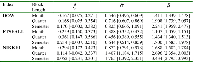
In Table 1 summary statistics detailing the first four moments, min and max values
and the Jarque-Bera normality test are given for the full distribution of returns and for
a subset of values incorporating 10 percent of the full sample. The latter analysis is to
investigate the tail behaviour of financial returns, as it this part of the distribution that
gives rise to catastrophic risk and our application of GEV. Overall, we find the mean
of upper and lower tail returns deviate substantially from the approximately zero
mean of the full distribution of returns, with the Nikkei exhibiting the largest
deviations. Moreover, daily risk is approximately 1% although some very large single
day returns occur.
INSERT TABLE 1 HERE
Standard financial time series properties are recorded for the tail and full distributions
namely, a lack of normality, due to excess skewness, and excess kurtosis. To
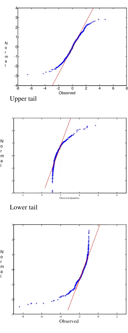
investigate this latter property in more detail, Figure 1 presents QQ plots of quantiles
of the observed distribution set against the normal distribution for both the full set of
distributions exhibit fat-tails. Second, the fat-tail characteristic becomes more
pronounced for the tail returns. These plots drive our application of the GEV and in
particular, the Fréchet GEV.
INSERT FIGURE 1 HERE
Turning to the extreme value analysis, maximum likelihood parameters of the fitted
GEV to the upper tails of the indexes are given in table 2. The dispersion parameter
values concur with the summary statistics of the tail distributions, indicating that the
Nikkei index fluctuates more than its counterparts. And as expected, the location and
dispersion estimates increase as interval size increases. As stated, the most important
parameter for modelling and distinguishing tail behaviour is the shape parameter. We
find all point estimates are positive, and generally there is support for the hypothesis
of returns converging to the fat-tailed Fréchet distribution at a 95% confidence levels.
Specifically, the fattest tail shape recorded is for the FTSE index at a quarterly
interval with a shape point estimate of 0.361. Variation in tail shape does occur
across markets, and interval of estimation, where no systematic pattern occurs. For
example, the shape parameter is reasonably constant across the intervals for the Dow
whereas it decreases for the Nikkei. This has implications for the modelling of
catastrophic risk where each asset should be modelled separately, and for different
frequencies.
INSERT TABLE 2 HERE
Taking the three EV parameters, we now estimate the catastrophic risk levels for a
99.9% confidence level and these are given in Table 3. This allows us to obtain
estimated 20-month, 20-quarter and 20-semester catastrophic risk levels for the upper
and lower tail of each index. These have an attractive inference with for example, a
20-month catastrophic risk level representing a level that we expect to exceed in one
month out of every twenty months on average. So for example, the 20-month
catastrophic risk level for the upper tail of the Nikkei index is 5.82% implying that
positive extreme price movements of this magnitude are expected in this market once
every 20 months on average.
INSERT TABLE 3 HERE
Some interesting findings are noted. Catastrophic risk increases as you increase the
interval size where investors would experience larger absolute returns from these
major markets. Furthermore, with the exception of the Dow for monthly blocks,
lower and upper catastrophic risk is similar and is within the respective confidence
intervals for each interval block. However in terms of identifying the riskiest market
at this interval, we find that the Nikkei exhibits the largest levels, and the FTSE
exhibits the smallest levels, of extreme returns.
An overall portfolio return is driven by these extreme catastrophic values as investor
performance is frequently the end result of a few exceptional trading days as most of
the other days only contribute marginally to the bottom line. Hence correct modelling
References:
Cotter, J. (2005) Tail Behaviour Of The Euro, Applied Economics, 37, 1 –14.
Cotter, J. (2004a) Extreme Risk in Futures Contracts, Applied Economic Letters,
Forthcoming.
Cotter, J. (2004b) Downside Risk For European Equity Markets, Applied Financial
Economics, 14, 707-716.
Cotter, J. and D.G. McKillop (2000) The Distributional Characteristics of a Selection
of Contracts Traded on the London International Financial Futures Exchange, Journal
of Business Finance and Accounting, 27, 487-510.
Dewachter, H. and G. Gielens (1999) Setting Futures Margins: The Extremes
Approach, Applied Financial Economics, 9, 173-181.
Embrechts, P., Klüppelberg, C., and T. Mikosch (1997) Modelling Extremal Events
for Insurance and Finance, Springer-Verlag, Berlin.
Kindleberger C. P. (2000) Manias, Panics and Crashes, 4th Edition, Wiley, New York.
Longin, F.M (2000) From value at risk to stress testing: The extreme value approach,
Acknowledgements: University College Dublin’s Faculty research funding is
Full series
Upper tail
Upper tail
[image:11.612.94.310.83.645.2]Lower tail
Figure 3. Q-Q plots of Dow Jones Industrial Average returns.
This figure plots the quantiles of the observed distribution against the normal distribution (straight line) for the full series and upper and lower 10 percent of returns.
-8 -6 -4 -2 0 2 4 6 8
-4 -3 -2 -1 0 1 2 3 4 Observed Quantiles N o r m a l
-8 -6 -4 -2 0 2
-3 -2 -1 0 1 2 3 Observed N o r m a l
-2 0 2 4 6 8
Table 1. Summary statistics for daily index series
Index Mean Std D Min Max Skew Kurt J-B
DOW 0.0524 1.06 -25.64 9.67 -3.74 92.32 1397123
Upper 1.76 0.76 1.12 9.67 4.14 33.55 17404
Lower -1.80 1.50 -25.64 -0.97 -10.36 154.85 408088
FTSEALL 0.0387 0.87 -11.91 5.70 -1.31 20.32 53380
Upper 1.45 0.59 0.98 5.70 3.28 18.83 5104
Lower -1.53 0.96 -11.91 -0.91 -6.04 55.85 51071
NIKKEI 0.0043 1.34 -16.14 12.43 -0.17 13.01 17453
Upper 2.39 1.17 1.40 12.43 3.23 20.12 5820
Lower -2.48 1.15 -16.14 -1.45 -4.93 50.80 41392
Table 2. Parameter estimates for upper tail of index series
Index Block
Length ξ
ˆ σˆ µˆ
DOW Month 0.167 [0.075, 0.271] 0.546 [0.495, 0.609] 1.411 [1.339, 1.478]
Quarter 0.168 [0.025, 0.354] 0.716 [0.607, 0.869] 1.908 [1.739, 2.057] Semester 0.170 [-0.002, 0.382] 0.825 [0.665, 1.091] 2.241 [1.959, 2.477]
FTSEALL Month 0.259 [0.150, 0.373] 0.388 [0.352, 0.432] 1.107 [1.059, 1.151] Quarter 0.361 [0.147, 0.586] 0.456 [0.389, 0.555] 1.434 [1.340, 1.513] Semester 0.214 [-0.007, 0.510] 0.644 [0.514, 0.859] 1.800 [1.585, 1.978]
NIKKEI Month 0.294 [0.172, 0.423] 0.872 [0.791, 0.973] 1.688 [1.582, 1.784] Quarter 0.114 [-0.042, 0.337] 1.407 [1.184, 1.715] 2.696 [2.354, 3.003] Semester 0.052 [-0.231, 0.301] 1.765 [1.392, 2.351] 3.434 [2.795, 3.993]
Table 3. Estimated catastrophic risk levels of index series
Index Tail Month Quarter Semester
DOW Lower 4.32 [3.71, 5.29] 6.47 [4.90, 10.09] 9.04 [6.05, 19.40]
Upper 3.51 [3.14, 4.07] 4.66 [3.92, 6.25] 5.45 [4.33, 8.40]
FTSE Lower 3.21 [2.80, 3.87] 4.07 [3.29, 5.97] 5.02 [3.63, 10.69]
Upper 2.84 [2.50, 3.39] 3.89 [3.03, 6.04] 4.47 [3.49, 7.87]
NIKKEI Lower 5.46 [4.77, 6.60] 7.09 [5.85, 9.71] 8.81 [6.62, 16.69]
Upper 5.82 [4.95, 7.28] 7.67 [6.38, 10.65] 9.10 [7.33, 14.59]