A Quick Classification Method of the Power Quality Disturbances

(1)

http://dx.doi.org/10.4236/eng.2014.67040

A Quick Classification Method of the Power

Quality Disturbances

Yi Tang1_{, Hao Liu}1,2

1_{School of Information and Electrical Engineering, China University of Mining & Technology, Xuzhou, China} 2_{NARI Group Corporation (State Grid Electric Power Research Institute), Nanjing, China}

Email: [email protected], [email protected]

Received 3 November 2013; revised 5 April 2014; accepted 20 April 2014

This work is licensed under the Creative Commons Attribution International License (CC BY). http://creativecommons.org/licenses/by/4.0/

Abstract

This paper introduces a quick classification method of the power quality disturbances. Based on analyzing the characteristics of different electrical disturbance signals in time domain, four tinctive features are extracted from electrical signals for classifying different power quality dis-turbances and then an automatic classifier is proposed. Using the proposed classification method, a PQ monitor of the classifying power quality disturbances is developed based on the TMS320F2812 DSP micro-processor. Semi-physical simulation, lab experiment and field measurement results have verified that this proposed method can classify single or complex disturbance signals effec-tively.

Keywords

Power Quality, Disturbance Classification, Noise

1. Introduction

(2)

2. The Analysis of Power Quality Disturbances in Time Domain

The general single-phase voltage signal can be expressed as the superposition of the fundamental wave voltage and the disturbance signals:

( )

(

)

(

)

(

)

( )

₍

₎

1 1

2 1

2 sin 2 sin 2 sin e s s1

n m

t t

h h s s s s

h s

u t U ω ϕt U h tω ϕ U ωt ϕ −γ − t t

= =

= + +

∑

+ +

∑

+ − (1)

where U1 is the RMS (root mean square) voltage with the system fundamental frequency; ω is the system fundamental angular frequency; ϕ1 is the initial phase angle; Uh is the hth harmonic RMS voltage; ϕh is the

hth harmonic initial phase angle; ωs is the angular frequency between harmonic waveforms and not an integer

multiple of the system fundamental frequency, for example, the frequencies of interharmonics and oscillatory transients; Us is the ωs RMS voltage with ωs angular frequency; ϕs is the initial phase angle of the ωs

angular frequency voltage; γs is the oscillatory transient attenuation constant. When γ =s 0, Us is the

in-terharmonic RMS voltage and when γ ≠s 0, Us is the oscillatory transients RMS voltage; ts is the starting

time; l(t) is the unit step function. Table 1 shows that characteristics of the disturbances which IEEE classified

[12]. All the simulation parameters in this paper are chosen from Table 1 randomly. In Equation (1), when U1 is stationary, equal to the rating value and

(

)

(

)

( )

₍

₎

2 1

2 sin 2 sin e s s 1 0,

n m

t t

h h s s s s

h s

U h tω ϕ U Iω ϕt −γ − t t

= =

+ + + − =

∑

Equation (1) represents the ideal voltage. So the voltage disturbance can be divided into two categories. One is the disturbances with the change of the U1 amplitude, including voltage sag, swell, interruption, under voltage, over voltage, fluctuation, flicker and so on. The other is the additive disturbances, including harmonics, oscilla-tory transients, impulse voltage, interharmonics and so on. From the aspect of disturbance duration, we can also divide the disturbances into two categories. One is stationary disturbance, including voltage fluctuation and flicker, under voltage, over voltage, continuous interruption, harmonics, interharmonics and so on. The other is transient disturbances, including voltage sag, swell, instantaneous interruption, oscillatory transients, impulse voltage and so on. So the power quality disturbances can be divided into four categories by time domain features, shown in Table 2.

For voltage sag, swell and interruption has the similar characteristics, the author only takes voltage sag as the analyzing object. The other two can also be identified by the method presented in this paper.

If u t

( )

in Equation (1) is multiplied by 2 sin

(

ω ϕt+ 1

)

, we can get:

( )

2 sin

(

1

)

1d 1i

( )

1un

( )

[image:2.595.129.492.491.716.2]

u t ∗ ω ϕt+ =u +u t +u t (2)

Table 1. Typical characteristics of power system disturbances.

Disturbances Typical spectral content Typical duration Typical voltage magnitude

Voltage sag 0.5 cycles - 1 min 0.1 - 0.9 pu

Fluctuation and flicker <25 Hz Intermittent 0.1% - 7%

Harmonics 0 - 100th_Hz _{Steady state} _{0% - 20%}

Oscillatory transients <5 kHz 0.3 - 50 ms 0 - 4 pu

Interharmonics 0 - 6 kHz Steady state 0% - 2%

Table 2. The categories of the voltage disturbance.

Voltage amplitude disturbances

Stationary Fluctuation and flicker, under voltage ,over voltage

Transient Voltage sag, swell, transient interruption

Additive disturbances

Stationary Harmonics, interharmonics

[image:2.595.127.470.514.626.2]

(3)

where, u1d =U1−U1cos 2

(

ωt+2ϕ1

)

, and 1 ₀ 1 d 1

T

d d

U =

∫

u t=U

(

)

{

(

)

(

)

}

1 1 1 1 1

2

cos 2 2 cos 1 cos 1

N

i h h h

h

u U ωt ϕ U h ω ϕt ϕ h ω ϕt ϕ

=

= + +

∑

_ − + − _− _ + + + _ , and ₁ ₁

0 d 0

T

i i

U =

∫

u t=

(

)

(

)

{

}

( )

₍

₎

1 1 1

1

cos cos e s s1

m

t t

un s s s s s s

s

u U Iω ω t ϕ ϕ Iω ω t ϕ ϕ −γ − t t

=

   

=

∑

_ − + − _− _ + + + _ − , and 1 ₀ 1 d 0

T

un un

U =

∫

u t≠

Equation (2) consists of three parts. First is DC component u1d. Second is an AC component u1i with an

integer multiple system frequency. Third is an AC component u1un with a non-integer multiple system

fre-quency. After a full cycle (0 - T) integral of the (2) we can see that U1i =0, and some AC components still exist

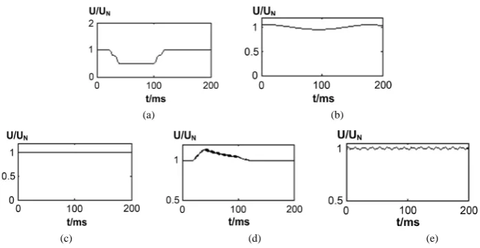
in U1un. Figure 1 is the curve of the full cycle integral of (2). In Figure 1(a) andFigure 1(b) only contain U1d.

Figure 1(c) contains U1d and U1i

(

U1i =0

)

. Figure 1(d) and Figure 1(e)contain U1d and U1un. For u1un

is the sine wave AC value of non-integer multiple system frequency, after a full cycle integral U1un ≠0. It

shows the existence of the sine wave AC disturbance of non-integer multiple system frequency. The simulation parameters of the following pictures are chosen in the range of Table 1.

The square of Equation (1) is:

( ) ( )

d i un

u t ∗u t =u + +u u (3)

The expanded formula of (3) is long, but also is consists of three parts: DC component ud, an AC

compo-nent u1i with an integer multiple system frequency, an AC component u1un with a non-integer multiple

sys-tem frequency. In it:

( )

2 ( )

₍

₎

2 2 2

1 0

2 1

d e s s 1

N m

T _{t t}

d d h s s

h s

U u t U t U U −γ − t t

= =

=

_∫

= +

∑

+

∑

− (4)

The curve of a full cycle integral of (3) is shown in Figure 2.

By comparing Figure 1and Figure 2, we can find that Figure 1(a) andFigure 1(b) are the same withFigure 2(a) and Figure 2(b) because there is no additive disturbance in the voltage sag and fluctuation and flicker. The harmonics is additive disturbance, so the Ud/UN in Figure 2(c) is larger than U1/UN in Figure 1(c). And the dif-

ference between them is the amplitude of the additive disturbance 2 2 N h h U =

∑

. The oscillatory transients and interharmonics are the additive disturbances. So the Ud/UN in Figure 2(d) and Figure 2(e) is larger than the U1/UN

in Figure 1(d)and Figure 1(e). And the difference is also the amplitude of additive disturbance ( )

₍

₎

2 2

1

e s s 1

m

t t

s s

s

U −γ − t t

=

−

∑

.

(a) (b)

(c) (d) (e)

(4)

(a) (b)

[image:4.595.125.474.81.261.2]

(c) (d) (e)

Figure 2. The curve of full cycle integral of (3). (a) Voltage sag; (b) Fluctuation and flicker; (c) Harmonics; (d) Oscillatory transients; (e) Interharmonics.

3. Basic Idea of the Classification of the Power Quality Disturbances

Though above analysis, some individual features of the power quality disturbance singles can be shown in time- domain:

1) Equation (2) has the effect of selecting system fundamental frequency. The DC component, which can be gotten by low pass filter from Equation (2), is the RMS voltage with system fundamental frequency, which is not affected by additive disturbance. And its change is equivalent to the amplitude disturbance of the RMS vol-tage (like volvol-tage sag, swell, transient interrupt, under volvol-tage, over volvol-tage, continuous interrupt, fluctuation, flicker and so on).

2) The DC component of Equation (3) is the geometric sum of the RMS voltage with system fundamental frequency and all other additive disturbance RMS voltages. So the geometric difference of the Equation (3) and Equation (2)’s DC component is exactly equivalent to the amplitude of the additive disturbance (like harmonics, oscillatory transients, impulse voltage and interharmonics).

3)Figure 1(d) and Figure 1(e)’s curves contain U1d and U1un.The component U1un exists usually because

of the existence of the interharmonics and the oscillatory transients which are non-integer system fundamental frequency sine wave signal. U1un≠0 indicates the existence of the interharmonics or oscillatory transients.

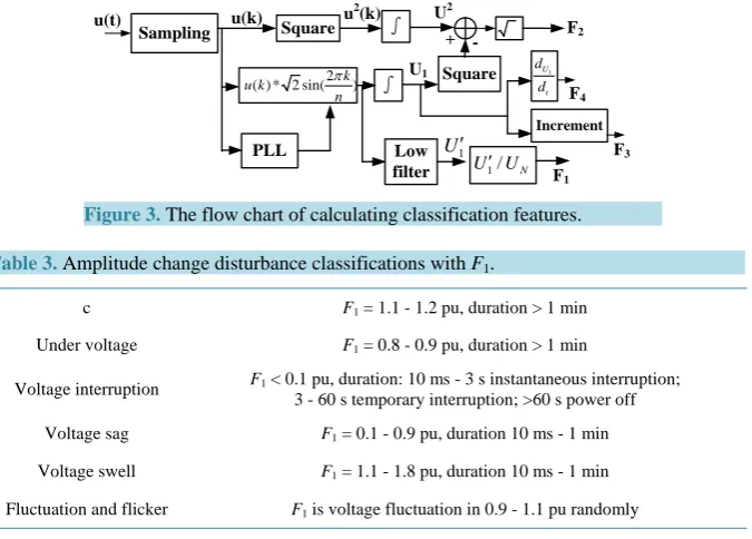
So, the next 4 features (F1 - F4) can be used to classify power quality single disturbances and the mixed dis-turbances can be considered as the “superposition” of the single disdis-turbances. The calculating flow chart of the 4 features is shown in Figure 3.

1) F1=U U1′ N is taken as a feature after Equation (2) is filtered by a low pass. Because of the (2)’s effect of

frequency selection, F1 is the system fundamental wave voltage amplitude variation value which is not affected by additive disturbance. It reflects the extent of the fundamental wave amplitude change. So the information of system fundamental RMS voltage change can be known from the extent of the F1 change. Then it can be used to identify whether there are the voltage sag, swell, instantaneous interruption, under voltage, over voltage, conti-nuous interruption, fluctuation and flicker in electrical singles (shown in Table 3).

2) 2

( )

2

( )

2

( )

2 1 1

1

100 N

k

F U k U k U k

N =

 

=

∑

_ − _ . N is the total sample points during the analysis period of time τ

(for F2 is used to detect stationary additive disturbances, the analysis period of time can be enlarged. This paper takes τ=2 s, 100 cycles). F2 is the RMS value of the additive disturbance during the analysis period of time

τ . If F2 >0, the additive disturbance must exist. If F2 is stationary, the disturbance must be harmonics and 2

F is equivalent to THD. F2>1.5 can be the threshold value of the harmonics and interharmonics.

3) If F2 >0, 3 1

( )

1

(

)

1

100

1

N

k

F U k U k

N =

=

∑

− − means the average increment of the U1un. It can be used to

(5)

Sampling Square

2 ( ) * 2 sin( k) u k

n π

PLL Low filter

∫

Square

F1

Increment

F2

F4

F3

u(t) u(k) u2(k) U2 + -U1

∫ Ut1

d

1

U′

1/ N

[image:5.595.132.470.86.328.2]

U′ U

Figure 3. The flow chart of calculating classification features.

Table 3. Amplitude change disturbance classifications with F1.

c F1 = 1.1 - 1.2 pu, duration > 1 min

Under voltage F1 = 0.8 - 0.9 pu, duration > 1 min

Voltage interruption F1 < 0.1 pu, duration: 10 ms - 3 s instantaneous interruption; 3 - 60 s temporary interruption; >60 s power off

Voltage sag F1 = 0.1 - 0.9 pu, duration 10 ms - 1 min

Voltage swell F1 = 1.1 - 1.8 pu, duration 10 ms - 1 min

Fluctuation and flicker F1 is voltage fluctuation in 0.9 - 1.1 pu randomly

and Figure 1(e)). Then value of F3 is much larger than that when only harmonics exist. The MATLAB simu-lation shows that when F3≥1, interharmonics exist; when F F3 2≥0.5, only interharmonics exist; when

3 2 0.5

F F < , both harmonics and interharmonics exist.

4) F4 =Max

{

U k1

( )

−U k1

(

−1

)

}

−F3. F4 is the maximum differential value of U1un. The characteristic

that the amplitude of instantaneous disturbance changes fast determines F4 a large number. But to stationary disturbance, F4 is small or even zero. The value of F4 can determine the instantaneous disturbances exist or not. The MATLAB simulation shows that the threshold can be 15. If F4 >15, the instantaneous disturbance exists; if F4 <15, no instantaneous disturbance exists. For instance, when F1 shows amplitude disturbance exists, if F4 >15, the disturbance should be instantaneous amplitude disturbance such as the voltage sag, swell, instantaneous interruption, and if F4 <15, the disturbance should be stationary amplitude disturbance such as under voltage, over voltage, fluctuation and flicker and when F1 shows no amplitude disturbance exists, if

4 15

F > , the disturbance must be the additive instantaneous disturbance such as oscillatory transient.

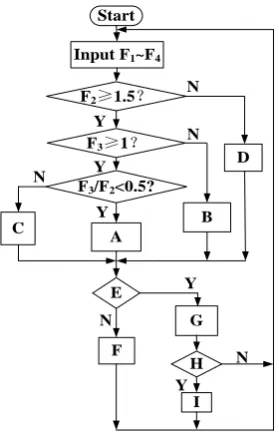
Table 4shows the simulation value of 5 single disturbances and 4 mixed disturbances. Figure 4 is the flow chart of the automate classification of the disturbances.

Disturbances can be classified into two categories: voltage amplitude disturbance and additive disturbance as shown in Table 2. F1 is used to identify whether voltage amplitude disturbances exist, and F2 is used to identify whether additive disturbances exist. F3 is used to identify whether (there is interharmonics in additive disturbances) interharmonics exist when F2>1.5. In the disturbances classification, it is very hard to identify the circumstance that both harmonics and interharmonics exist. The interharmonics have effect on F2 and F3. When the interharmonic disturbance is heavy, F3 is large, and F2 is large, too. So F F3 2 is relatively steady. When harmonics and interharmonics both exist, F F3 2 is smaller than that when only interharmonics exist. A lot of simulation results indicate that F F3 2 can identify the circumstance that both harmonics and in-terharmonics exist correctly. F4 is used to identify whether transient disturbances exist.

4. Discussion

Comparing with the other power quality disturbance classification methods using some kinds of transforms, the method presented by this paper has advantages as follows:

(6)

[image:6.595.229.369.84.302.2]

Figure 4. The flow chart of the automate classification. A: Har- monics + Interharmonics; B: Harmonics; C: Interharmonics; D: No stationary additive disturbance; E: F1=Constant≈1 pu?; F: Identify the amplitude disturbances by F1; G: No amplitude dis-

turbance; H: F4>15?; I: Osillatory transients.

Table 4. The simulation value of the features.

The disturbances The disturbance parameters F2 F3 F4

Fluctuation and flicker Amplitude: 0.95 - 1.05 0.68 0. 91 1.96

Voltage sag Sag amplitude: 0.5 pu 0.49 0. 40 38.66

Harmonics *₅th_{4%; 7}th_3% _5.0 ₀ ₀

Oscillatory transients Ms = 0.8 pu, fs= 1025 Hz; Us = 0.1 0.49 0.22 59.95

Interharmonics f = 125 Hz, amplitude 2% 1.99 1.27 1.78

Voltage sag and harmonics 0.5 pu, 5th_{4%; 7}th_3% _5.41 _{0. 40} _39.45

Fluctuation and harmonics Amplitude: 0.95 - 1.05; 5th_{4%; 7}th_3% _5.05 _{0. 91} _1.31

Harmonics and oscillatory transients 5th_{4%; 7}th_3%,_γ

s = 0.1, Us = 0.8 pu, fs = 1025 Hz 5.34 0. 22 59.92

Harmonics and interharmonics 5th_{4%; 7}th_3%;_f

s = 125 Hz, Us = 2% 5.37 1.27 1.73

2 1.5

F ≥ and F3<1, only harmonics exist; if F2≥1.5, F3≥1 and F F3 2≥0.5, only interharmonics exist; if F2≥1.5, F3≥1 and F F3 2<0.5, both harmonics and interharmonics exist.

2) The features extracted from one disturbance won’t change a lot for the existence of the other disturbance. This is shown clearly in Table 4. For example, when the voltage sag and harmonics both exist, F1 which is used to identify voltage sag won’t change for the existence of harmonics. And F2 (only harmonics exist,

2 5.0

F = ), which is used to identify harmonics changes a little by the existence of voltage sag (harmonics + vol-tage sag, F2 =5.41). When the oscillatory transients exist in harmonics, F2 increases a little (from 5.0 to 5.23). The harmonics and interharmonics are both additive disturbances, so F2 is the approximate geometric

summation of their amplitude ( 42+32+22 =5.39, the simulation result in Table 4 is 5.37). For another example, F4 which is used to identify transient voltage sag

(

F4 =38.66

)

and oscillatory transients

(

F4=59.95

)

will not change a lot for the existence of harmonics (voltage sag + harmonics, F4=39.45; oscillotary +

har-Start

Input F1~F4

F2≥1.5？

F3≥1？

F3/F2<0.5?

A

E

F

D

B C

G

H

I N

Y

N Y

Y N

N

N Y

[image:6.595.113.497.392.571.2]

(7)

monics, F4=59.92). This characteristic of the features is the key of the classifying the mixed disturbances. For the idea of this paper considers the mixed disturbances as the “superposition” of the single disturbances. For the characteristics above, all single or mixed disturbances can be classified correctly by simple classifying program, and the classifying results won’t conflict and are definitive.

3) The classifying features have clear physical meanings. So it profits the evaluation of the power quality dis-turbance. The physical meaning of F1 is the per unit value of the system fundamental RMS voltage, so the am-plitude of all the voltage amam-plitude disturbances can be gained from F1. And the starting time tq and the

end-ing time tz of the transient amplitude disturbance can also be gained from F1 (shown in Figure 1). The physical meaning of F2 is the content of the additive disturbances. So F2 gives the content of the harmonics and interharmonics accurately. The oscillatory amplitude and the attenuation constant of the oscillatory tran-sients can be gained by fitted method from Figure 2(d).

4) The calculating time is much less, and profits to be used in real-time power quality disturbance classifica-tion.

5) The features extracted are low-pass filtered or the full cycle integral values, so it has good ability of noise proof.

5. Verifications

Using the proposed power quality disturbance classification method, a PQ monitor is developed based on the TMS320F2812 DSP micro-processor. Semi-physical simulation, lab experiment and field measurement results have verified the proposed method.

5.1. Semi-Physical Simulation Results

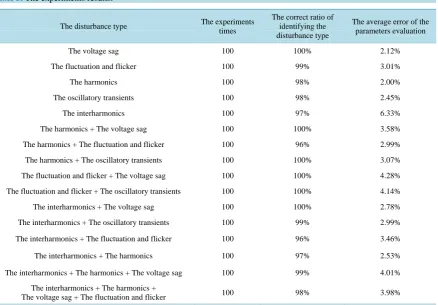
[image:7.595.100.539.416.721.2]

The authors use D space semi-physical experiment platform as the disturbance signal generator. The PQ monitor samples the signals generated by D space, identifies disturbances and evaluates their parameters. Table 5 shows that it identifies the disturbance types correctly and evaluates their parameters accurately.

Table 5. The experiments results.

The disturbance type The experiments times

The correct ratio of identifying the disturbance type

The average error of the parameters evaluation

The voltage sag 100 100% 2.12%

The fluctuation and flicker 100 99% 3.01%

The harmonics 100 98% 2.00%

The oscillatory transients 100 98% 2.45%

The interharmonics 100 97% 6.33%

The harmonics + The voltage sag 100 100% 3.58%

The harmonics + The fluctuation and flicker 100 96% 2.99%

The harmonics + The oscillatory transients 100 100% 3.07%

The fluctuation and flicker + The voltage sag 100 100% 4.28%

The fluctuation and flicker + The oscillatory transients 100 100% 4.14%

The interharmonics + The voltage sag 100 100% 2.78%

The interharmonics + The oscillatory transients 100 99% 2.99%

The interharmonics + The fluctuation and flicker 100 96% 3.46%

The interharmonics + The harmonics 100 97% 2.53%

The interharmonics + The harmonics + The voltage sag 100 99% 4.01%

The interharmonics + The harmonics +

(8)

The authors give three types of disturbances: the voltage sag, the voltage sag plus harmonics, the fluctuation plus harmonics plus interharmonics plus voltage sag to present 5 single disturbances and 11 mixed disturbances.

1) The voltage sag

[image:8.595.157.441.409.538.2]

In the following tables the same symbols have the same meanings.

Table 6 doesn’t give the true or false results because the PQ monitor gives the correct results every time. Ta-ble 6 shows that the PQ monitor can evaluate the voltage sag parameter very well. The relative error is a little big when the voltage sag amplitude is close to the voltage sag threshold value, but the absolute error is not big.

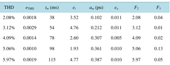
2) The voltage sag plus harmonics

The authors do not show the identifying results in Table 7, for all harmonics plus voltage sag are identified by the PQ monitor correctly. Table 7 shows that the superposed disturbance doesn’t make the features change a lot, which means the features F2 and F3 are relatively independent. The identifying results and the parameters evalu-ation are not affected by the superposition of the disturbances.

3) The fluctuation plus harmonics plus interharmonics plus voltage sag

Table 8 shows that the addition of the fluctuation and flicker affects the feature F2 a little, but doesn’t affect the feature F3. The big amount of harmonics may blanket the existence of interharmonics, because the identify-ing term of the harmonics plus interharmonics is F3/F2 > 0.5.

5.2. Lab Experiment Results

A lab experiment circuit is shown as Figure 5. When the switch S is turned on, there is voltage sag on R1. The voltage signal u1 is sampled by the PQ monitor and the oscilloscope.

U = 380 V, R1 = 1 kΩ, R2 = 2 kΩ, R3 = 3.9 Ω. S is an AC contact. FU is a fuse. When S is turned on and the current of the FU branch is large enough, the FU will blowing out and the branch will be cut off. Then there will be a voltage sag in u1 as shown in Figure 5(b).

The experiment results shown in Table 9 indicate that the PQ monitor can identify disturbances correctly and evaluate the voltage sag lasting time and amplitude accurately.

Table 6. The experiments results of voltage sag.

tm(ms) ts(ms) et am(pu) as(pu) ea

35 40 5 0.112 0.1 0.012

53 60 7 0.211 0.2 0.011

77 80 3 0.305 0.3 0.005

98 100 2 0.360 0.35 0.01

116 120 4 0.389 0.40 0.011

138 140 2 0.447 0.45 0.003

tm: The voltage sag lasting time measured by the PQ monitor; ts: The setting time of the

vol-tage sag lasting time; et: The error between time 1 and time 2; am: The voltage sag amplitude

measured by the PQ monitor; as: The setting amplitude of voltage sag amplitude; ea: The error

[image:8.595.157.440.601.709.2]

between amplitude 1 and amplitude 2.

Table 7. The experiments results of harmonics plus voltage sag.

THD eTHD tm(ms) et am(pu) ea F2 F3

2.08% 0.0018 38 3.52 0.102 0.011 2.08 0.04

3.12% 0.0029 54 4.76 0.212 0.011 3.12 0.01

4.09% 0.0014 78 2.60 0.307 0.005 4.09 0.02

5.06% 0.0010 98 1.93 0.361 0.010 5.06 0.13

5.97% 0.0019 115 4.77 0.387 0.010 5.97 0.05

(9)

[image:9.595.94.535.101.496.2]

Table 8. The experiments results of voltage fluctuation plus harmonics plus interharmonics plus voltage sag.

The disturbance parameters F2 F3 Results Remarks

Fluctuation modulating wave amplitude 0.02, frequency 6 Hz; interharmonics content 2%,frequency 125 Hz;

harmonics THD 2%; voltage sag amplitude 0.4 pu

4.72 3.75

Voltage Fluctuation plus harmonics plus interharmonics

plus voltage sag

4.80 3.80

Voltage fluctuation plus harmonics plus interharmonics

plus voltage sag

4.91 3.82

plus voltage sag

4.98 3.80

plus voltage sag

3.12 1.07 Voltage fluctuation plus harmonics plus voltage sag

When the interharmonics content is lower than 1%, and the harmonics content is large, the error is a little large

4.21 3.68

plus voltage sag

5.25 3.71

plus voltage sag

7.27 3.75

plus voltage sag

4.05 3.69

plus voltage sag

4.11 3.70

[image:9.595.99.501.493.594.2]

plus voltage sag

Table 9. The voltage sag experiments results comparison table.

Identifying results tm (ms) tom (ms) et am (pu) aom (pu) ea

Voltage sag 100 102 2 0.842 0.854 0.012

Voltage sag 102 105 3 0.838 0.833 0.005

Voltage sag 101 103 2 0.857 0.872 0.015

Voltage sag 108 110 2 0.813 0.801 0.012

Voltage sag 113 114 1 0.839 0.825 0.014

a: Error means the difference between values evaluated by PQ monitor and ones measured by the oscilloscope. For the oscilloscope measured value has error itself, but here, no error is considered. The meaning of error in the other tables is the same.

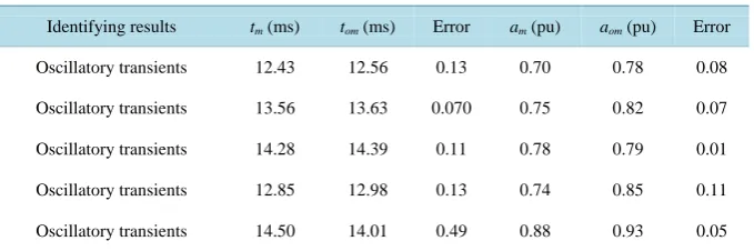
5.3. Field Measurement Results

A PQ monitor is equipped to a steel pipe factory substation to monitor the harmonics disturbance and the oscil-latory transient disturbances. The results are shown inTable 10 and Table 11.

The field monitoring results in Table 10show that the PQ monitor identifies harmonics correctly and eva-luates the THD accurately.

(10)

u

S R1

R2

R3

u1

FU

[image:10.595.144.446.81.212.2]

(a) (b)

Figure 5. The voltage sag experiment. (a) The voltage sag experiment circuit; (b) The waveform of u1.

[image:10.595.185.414.253.389.2]

Figure 6. The three phase voltage waveform of capacitors switching in Shi-Qiao substation.

Table 10. The harmonics experiments results comparison table.

Identifying results THDm THDom Error

Harmonics 4.2% 4.4% 0.0020

Harmonics 5.0% 5.2% 0.0020

Harmonics 4.8% 5.0% 0.0020

Harmonics 4.5% 4.8% 0.0030

Harmonics 5.7% 6% 0.0030

THDm: THD measured by the PQ monitor; THDom: THD measured by the oscilloscope.

Table 11. The experiments results of oscillatory transient in Shi-Qiao substation.

Identifying results tm (ms) tom (ms) Error am (pu) aom (pu) Error

Oscillatory transients 12.43 12.56 0.13 0.70 0.78 0.08

tom: The oscillatory transients lasting time measured by the oscilloscope; aom: The oscillatory transients amplitude

measured by the oscilloscope.

300 200 100

0.02 0.1 0.18

200 400

[image:10.595.129.469.435.547.2] [image:10.595.130.470.586.699.2]

(11)

The author takes one phase wave to analyze (the purple one). The field experiment results are shown in Table 11.

Table 11 shows that the PQ monitor identifies the oscillatory transients correctly and evaluates their parame-ters accurately. The difference between the values evaluated by the PQ monitor and ones measured by oscillos-cope is small.

6. Conclusion

Comparing with analyzing power quality disturbance signals in frequency domain, the method presented by this paper has some advantages. First, if one feature or some features satisfied some conditions, a disturbance or mixed disturbances can be sure. That is to say, the disturbance classification would not be probable, but be de-finitive. Second, the features extracted won’t change a lot for the existence of the other disturbances. This cha-racteristic is the key of classifying the mixed disturbances. Third, the features have clear physical meanings. So it profits the evaluation of the disturbance parameters.

References

[1] Heydt, G.T., Fjeld, P.S., Liu, C.C., et al. (1999) Applications of the Window FFT to Electric Power Quality Assess-ment. IEEE Transactions on Power Delivery, 14, 1411-1416. http://dx.doi.org/10.1109/61.796235

[2] Gaing, Z.-L. (2004) Wavelet-Based Neural Network for Power Disturbance Recognition and Classification. IEEE Transactions on Power Delivery, 19, 1560-1568. http://dx.doi.org/10.1109/TPWRD.2004.835281

[3] Ece, D.G. and Gerek, O.N. (2004) Power Quality Event Detection Using Joint 2-D-Wavelet Subspaces. IEEE Transac-tions on Instrumentation and Measurements, 53, 1040-1046. http://dx.doi.org/10.1109/TIM.2004.831137

[4] Chilukuri, M.V. and Dash, P.K. (2004) Multiresolution S-Transform-Based Fuzzy Recognition System for Power Quality Events. IEEE Transactions on Power Delivery, 19, 323-330. http://dx.doi.org/10.1109/TPWRD.2003.820180

[5] Gaouda, A.M., Salama, M.M.A., Sultan, M.K. and Chikhani, A.Y. (1999) Power Quality Detection and Classification Using Wavelet-Multiresolution Signal Decomposition. IEEE Transactions on Power Delivery, 14, 1469-1476. http://dx.doi.org/10.1109/61.796242

[6] Santoso, S., Powers, E.J., Grady, W.M. and Hofmann, P. (1996) Power Quality Assessment via Wavelet Transform Analysis. IEEE Transactions on Power Delivery, 11, 924-930. http://dx.doi.org/10.1109/61.489353

[7] Dash, P.K., Panigrahi, B.K. and Panda, G. (2003) Power Quality Analysis Using S-Transform. IEEE Transactions on Power Delivery, 18, 406-411. http://dx.doi.org/10.1109/TPWRD.2003.809616

[8] Stockwell, R.G., Mansinha, L. and Lowe, R.P. (1996) Localization of the Complex Spectrum the S Transform. IEEE Transactions on Signal Processing, 44, 998-1001. http://dx.doi.org/10.1109/78.492555

[9] Axelberg, P.G.V., Gu, I.Y.-H. and Bollen, M.H.J. (2007) Support Vector Machine for Classification of Voltage Dis-turbances. IEEE Transactions on Power Delivery, 22, 1297-1303. http://dx.doi.org/10.1109/TPWRD.2007.900065

[10] Mishra, S., Bhende, C.N. and Panigrahi, B.K. (2008) Detection and Classification of Power Quality Disturbances Us-ing S-Transform and Probabilistic Neural Network. IEEE Transactions on Power Delivery, 23, 280-287.

http://dx.doi.org/10.1109/TPWRD.2007.911125

[11] Zhao, F.Z. and Yang, R.G. (2007) Power-Quality Disturbance Recognition Using S-Transform. IEEE Transactions on Power Delivery, 22, 944-950. http://dx.doi.org/10.1109/TPWRD.2006.881575