Estimating the Income Reporting Function for the Self Employed

Munich Personal RePEc Archive

Estimating the Income Reporting

Function for the Self-Employed

Tedds, Lindsay

University of Victoria

July 2007

Online at

https://mpra.ub.uni-muenchen.de/39784/

Estimating the Income Reporting Function for the Self-Employed1

Lindsay M. Tedds

School of Public Administration, University of Victoria PO Box 1700 STN CSC, Victoria, BC, Canada, V8W 2Y2

Phone: 250-721-8068, Email: [email protected]

This version: July 2007

Abstract

There is considerable interest in measuring the underground economy using microeconomic data. One such method estimates income under-reporting by households by assuming a known, parametric form of the Engel curve and making the further parametric assumption that households under-report their income by a constant fraction, independent of income. This paper proposes a nonparametric approach which avoids functional form restrictions and enables the reporting function to vary across income levels and household characteristics. I illustrate by estimating the effect of the Canadian Goods and Services Tax on income under-reporting.

Keywords: Underground Economy, Income Under-reporting, Nonparametric Estimation, Engel Curve

JEL Classification: C14, D12, O17

1

1. INTRODUCTION

There has been a recent resurgence in interest in measuring the underground economy

and this interest has been stimulated predominantly by the perception that the underground

economy is sizeable and growing. In broad terms, the phrase “underground economy” refers to

output that is produced and income that is generated by agents who hide this fact from

authorities. Knowledge of the size and structure of the underground economy is important for a

number of reasons. First, because underground activities are unmeasured, they are not taken into

account in the information-set that is used to assist economic policy-makers. Second, the

underground economy effectively re-distributes both income and wealth in ways that are not

necessarily consistent with the re-distributional goals of the taxation system. Third, the shortfall

in income-reporting that is associated with underground activities leads to an erosion in the tax

base and tax revenue with subsequent implications for both public expenditure and taxation

policies. Finally, enforcement activities are unlikely to be successful (and may have counter

productive consequences) without detailed knowledge of the characteristics and types of

activities of underground economy participants.

To date, research that seeks to measure the underground economy has predominately

employed macro-methods.2 These macroeconomic measures, however, have been criticized for not being consistent with modern economic models of consumer behaviour, employing flawed

econometric techniques, producing unreliable estimates, and providing limited guidance to

policy makers (Thomas 1999). In particular, the macro-methods developed to date do not

provide any information regarding the characteristics of those participating in the underground

2

economy. In order to obtain this type of information, a method that utilizes microeconomic data

is required.

One such approach, popularized by Pissarides and Weber (1989) and modified by

Lyssiotou et al. (2004), utilizes household income and expenditure data to estimate the degree of

income under-reporting (i.e. the amount by which household income should be scaled upwards

to obtain true, or actual, income as opposed to reported income). The basic principle of this

Expenditure-Based Method is that true household income can be imputed from reported

household expenditures. The method is premised on variations of several key assumptions,

namely: the reporting of expenditures on some items by all households is accurate; those who

report zero self-employment income report income accurately while those who report non-zero

self-employment income may under-report; and the marginal propensity to consume out of

unreported income is equal to the marginal propensity to consume out of reported income.

Actual, or true, self-employment income is then imputed by comparing the expenditure levels of

households with positive self-employment income to the expenditure-income bundles of

households with zero self-employment income and similar characteristics. In practice, the

method is implemented by estimating reliable expenditure functions (i.e. Engel curves) for wage

earners that are then inverted to estimate true income for the self-employed.

Previous studies have implemented the Expenditure-Based Method using highly

parametric restrictions on: (1) an Engel curve (Pissarides and Weber 1989) or a system of Engel

curves (Lyssiotou et al. 2004); and (2) an income reporting function. These restrictions imply

that households under-report their income by a constant fraction, independent of income. There

is no empirical evidence that supports this restriction and little, if anything, is actually known

implementing the Expenditure-Based Method. In particular, the parametric restrictions are

relaxed and a nonparametric approach to the measurement of income under-reporting is

explored.

Specifically, a two-step approach to estimating a variable-with-income reporting function

is proposed, within the framework of the Expenditure-Based Method. The approach is

essentially as follows. First, a nonparametric inverse food Engel curve is estimated for the

sample of households that report zero self-employment income, to obtain an estimate of true

income given (accurately) reported expenditures for every household in the sample (including

those with employment income). Second, the nonparametric reporting function for

self-employment income for households that report positive self-self-employment income is estimated.

This approach improves on the implementation of the Expenditure-Based Method by minimizing

the number of assumptions required for estimation. More particularly, the proposed framework

avoids the usual functional form restrictions and enables the reporting parameter to vary across

income levels.

The approach is illustrated by estimating the effect of the Canadian Goods and Services

Tax (GST) on income under-reporting by married households with self-employment income. It

is often argued that the implementation of this broadly based consumption tax increased the

incentives and opportunities for tax evasion (e.g. Spiro 1993, and Hill and Kabir 1996) though

the Government of Canada maintained that it would reduce the scope the tax evasion. The

empirical analysis uses the Canadian Family Expenditure Survey (FAMEX), which contains

household level information about income and expenditures.

Overall, this refinement to the Expenditure-Based Method produces results that

particular, the gap between true and reported self-employment income is larger for households at

the lower end of the self-employment income distribution. This result supports the fundamental

results of Reinganum and Wilde (1985, 1986) that “…taxpayers with greater true income

under-report less than those with lower true income…” (Reinganum and Wilde 1986, p. 741). Possible

explanations of this finding are that households with more self-employment income may think

they are more likely to be audited by the authorities, face higher utility costs if they are caught,

and/or disproportionately benefit from legal tax avoidance (e.g. by exploiting various tax credits

or loopholes). It is also found that some self-employed households, notably those households at

the upper end of the self-employment income distribution, over-report their income. The

parametric restrictions imposed previously masked this possible behaviour. Overall, the

aggregate results neither support the hypothesis that the GST increased tax evasion nor the claim

by the Canadian federal government that the GST would reduce tax evasion, at least for the

self-employed.

The remainder of this paper is organized as follows. First, estimating income

under-reporting from micro data is discussed, including a brief overview of the literature and details

regarding the nonparametric approach proposed by this paper. The application of the approach is

then described, including a description of the data, implementation details of the nonparametric

approach (e.g. kernel and bandwidth selection), the results, and a discussion regarding the

2. ESTIMATING INCOME UNDER-REPORTING FROM MICRO DATA

2.1.Previous Approaches

In this section, attention is focused on two critical aspects of the empirical work in this

paper with the view of placing the empirical strategy in context. These aspects concern: (1)

functional form restrictions; and (2) the treatment of permanent income.

2.1.1. Functional Form Restrictions

A critical aspect of the empirical work in this area is the specification of the expenditure

and reporting functions. The pioneering work in the development of the Expenditure-Based

Method was conducted by Pissarides and Weber (1989).3 First, they categorize households as either being self-employed or wage earning. Second, they specify a log-log (in expenditures and

income) form for the expenditure equation (i.e. the constant elasticity Engel curve) that is used to

estimate the parameter θ in the linear reporting function for self-employed households, defined

as

SE SE y

y*  (1)

where y*_SE represents true self-employment income, y_SE denotes reported self-employment

income, and θ is assumed to be > 1. This method of estimating income under-reporting consists

of two steps. First, an expenditure function is estimated for wage earners. Second, the

expenditure function is inverted to calculate θ, the amount by which reported self-employment

income must be scaled up by in order to obtain true self-employment income.

3

Figure 1 provides a graphical representation of the approach. Constant-elasticity Engel

curves for wage (or employee) and self-employed households are shown. A self-employed

household reports expenditures, E*, and income, Y, but the reported level of expenditures is

actually consistent with true income, Y*. The amount by which reported income must be scaled

up to obtain true income is calculated by taking the ratio of the distance 0Y*/0Y which is

equivalent to the parameter θ in equation (1) above. As the Engel curve for the self-employed is

assumed to be parallel to that of wage earners, the distance is the same for every household (i.e.

the reporting parameter is constant).

Lyssiotou et al. (2004) propose a systems approach to the Expenditure-Based Method.

They specify a system of Engel curves of quadratic-in-(log)income Working-Leser form. They

assume that durable and nondurable goods are separable and base their demand system on

nondurable goods only, namely: food, alcohol, fuel, clothing, personal goods/services, and

leisure goods/services. Lyssiotou et al. (2004) maintain the specification of the linear reporting

function given in equation (1) above but avoid classifying households as either wage earners or

self-employed.4

The functional form for the Engel curve that is specified by Lyssiotou et al. (2004) raises

two concerns. First, there is an implicit assumption of the Expenditure-Based Method that the

Engel curve(s) employed in the estimation must be monotonic in income. In reference to Figure

1, if this critical assumption is violated, then a unique value of true income associated with a

4

particular level of expenditures may not exist. The quadratic-in-(log)income Working-Leser

form of the Engel curve specified by Lyssiotou et al. (2004) is not necessarily consistent with the

monotonicity assumption, with particular goods, notably alcohol and clothing, known to violate

this assumption (Banks et al. 1997). Second, the quadratic-in-(log)income Working-Leser form

of the Engel curve is not invertible over all values due to the presence of asymptotes. While the

presence of asymptotes is not a concern under the structure imposed by Lyssiotou et al. (2004)

-the system of Engel curves is not (implicitly) inverted over all data points - it underscores -the

likelihood that the estimates are influenced, in whole or in part, by the parametric restrictions.

More generally, this approach still assumes a parametric Engel curve, albeit one that is

more widely accepted than that implied by earlier constant-elasticity assumption. Perhaps more

importantly, this approach continues to assume that households under-report their income by a

constant fraction, independent of income. In fact, little is known about the form of the reporting

function and it is plausible that under-reporting will differ with income and household

characteristics. This paper proposes a nonparametric approach which avoids functional form

restrictions. The proposed method also works directly with an inverse Engel curve, avoiding

problems associated with inversion, and continues with the tradition of the single equation

approach. The single equation approach also allows the analysis to be restricted to a good for

which the Engel curve is widely acknowledged to be monotonic in income.

2.1.2. Permanent Versus Transitory Income

There is a general belief that households base expenditures on permanent rather than

transitory income. This implies that households save when they have positive transitory income

implemented using transitory, or annual income, this may lead to biased estimates of income

under-reporting. Pissarides and Weber (1989) acknowledge that permanent income is the

measure of income that influences consumption decisions but stop short of requiring their

expenditure function to conform exactly to the permanent income hypothesis, perhaps because

the dataset used in their analysis (1982 British Family Expenditure Survey) did not contain

information regarding household savings behaviour. They indicate that “…for given permanent

income, the measured income of the self-employed may be more variable than the measured

income of employees in employment. If this is correct, our measure of income under-reporting

by the self-employed will have to be adjusted accordingly.” (Pissarides and Weber 1989, pp. 20)

Empirically, they implement this assumption by treating reported income as endogenous and

then using instrumental estimation, which “…enables an independent estimate of the residual

variance of reported income for each group which is exploited in the calculation of income

under-reporting.” (Pissarides and Weber 1989, pp. 22)

Whether Pissarides and Weber’s (1989) Two-Stage Least Square (2SLS) approach is

preferred to Ordinary Least Squares (OLS) depends on the quality of the instruments. Datasets

that contain information on household expenditures and income may not contain relevant and

suitable instrumental variables required for this analysis. Further, the approach requires the

researcher to make additional and somewhat arbitrary assumptions which restrict the analysis.

As a result, an alternative approach which addresses the issue of permanent income is desirable.

2.2. A Nonparametric Approach

As outlined above, to date, the Expenditure-Based Method has been implemented by

estimating Engel curves which are implicitly or explicitly inverted to obtain an average estimate

of income under-reporting. A more direct approach to estimating income under-reporting is to

utilize an inverse Engel curve (i.e. with income taking on the role of the dependent variable) and

nonparametric methods. Within the framework of the Expenditure-Based Method, a two-step

approach to estimating a variable-with-income reporting function is proposed that responds to

the concerns raised in the previous section.

The first step nonparametrically estimates an inverse Engel curve, which can be

consistently estimated for households that report zero self-employment income, to obtain true

income for all households. The second step nonparametrically estimates the reporting function

for households with positive self-employment income. The use of nonparametric methods has

three advantages. First, it enables the reporting function to vary across income levels and

household characteristics. Second, it avoids functional form restrictions on the Engel curve.

Third, within this framework it is also possible to test the null hypothesis that the reporting

function is linear, as has been assumed in the previous literature.

Estimating Engel curves using nonparametric techniques is quite common and

demographic household characteristics, used to account for observable heterogeneity, are often

included by specifying a partially linear additive semi-parametric specification using the

Yatchew (1997) or Robinson (1988) approach. However, “restrictions from consumer theory are

not innocuous both on the form of the Engel curve relationship and on the way in which

observable heterogeneity (demographics in our case) can enter.” (Blundell et al. 1998, pp. 436)

demographic composition and income that underlies the partially linear semiparametric model

implies strong and unreasonable restrictions on behaviour.” (Blundell et al. 1998, pp. 459)

Rather, to be consistent with consumer theory, the demographics that enter the Engel curve

specification must also scale the income term. The nonparametric estimation strategy proposed

here cannot be implemented if income and demographic terms enter non-additively, hence,

semiparametric estimation was not pursued. Instead, estimation is conducted separately on an

identified homogenous sub-population (i.e. married couples without dependent children present

in household).5

To achieve estimation, some initial assumptions are required. The three fundamental

assumptions of Pissarides and Weber (1989) are maintained and classifying households as either

self-employed or not is avoided, following Lyssiotou et al. (2004). First, food expenditures are

used in the analysis and it is assumed that the reporting of food expenditures by all households is

accurate.6 Second, only self-employment income can be under-reported.7 Third, the marginal

5

This is not to say that a semi-parametric approach cannot be pursued within the framework proposed but is beyond the scope of this paper.

6

The arguments for using food as opposed to any other commodity or group of commodities are that: there is no social stigma associated with food consumption which could cause expenditures to be reported inaccurately (counter examples would include tobacco and alcohol); food expenditures are more likely to be reported accurately by households participating in the underground economy since individual expenditures on food are small and are unlikely to rouse suspicion; tastes for food are more likely to be uniform across employment groups and over time; it is very difficult for a household to postpone food consumption; most food purchases cannot be included as a business expense; and, the food Engel curve is widely acknowledged to be monotonic. However it should be noted that the self-employed in many countries are able to write-off for tax purposes food that is consumed in restaurants much more easily than wage employees.

7

propensity to consume out of unreported income is constrained to be equal to the marginal

propensity to consume out of reported income.8

The estimation strategy is as follows. The object of interest is true household

self-employment income, y*_{SE h,} , which is assumed to be a function of reported household

self-employment income, y_{SE h,} , plus a white noise disturbance term:

*

, , ,

( _{SE h}| _{SE h}, 1] ( _{SE h}) _h

E y y d   f y  (2)

where h denotes an individual household and d is a dummy variable that takes a value of one if

the household reports any self-employment income.

The first stage of the procedure is to nonparametrically estimate an inverse Engel curve to

obtain true (permanent) income given (accurately) reported expenditures. The inverse Engel

curve expresses income, in this case permanent income, for reasons discussed above, as a

function of expenditures. For this exercise, the nonparametric representative of the inverse

Engel curve is given by:

, ( )

p

h h TOTAL h

y h x  (3a)

where xh represents household reported (and assumed to be true) food expenditures, h is a

white noise disturbance term, and y_{TOTAL h}p _, represents true (reported plus unreported) total

permanent household income, defined as

taxes. The extent that this assumption is not valid will lead to the resulting estimate of the degree of under-reporting to be biased toward zero.

8

*

, ,

, .

p

SE h OTH h h TOTAL h

y  y y  A (3b)

,

OTH h

y refers to household reported (and assumed to be accurately reported) other income and

h A

 indicates household net change in financial assets and liabilities (a household that has

positive (negative) transitory income will save (dissave) the additional money and Ah>0 (<0)).

By assumption, xh is accurately observed for all households but _, p TOTAL h

y is only

accurately observed for those households that have zero self-employment income

(y*_{SE h,} =y_{SE h,} =0). This implies that h(xh) can be consistently estimated for households that

report zero self-employment income. The fitted values from the first stage regression, ˆ(h x_h), for

households that report zero self-employment income are used to obtain an accurate estimate of

total permanent income for households with positive self-employment income based on food

expenditures. As a result, consistent estimates of total permanent household income, ˆ(h x_h), are

obtained for every household.

As indicated in equation (3b) above, total permanent household income is comprised of

three elements, namely the household’s: true self-employment income, (y*_{SE h,} ); reported other

income, (y_{OTH h,} ); and net change in financial assets and liabilities, (Ah). If yOTH h, is

subtracted from and Ah is added to the estimate of total permanent household income obtained

in the first step, ˆ(h x_h), one obtains an estimate of true self-employment income, y*_{SE h,} , for those

households that report positive self-employment income. That is, y*_{SE h,} can be calculated as

*

, ˆ( ) , .

SE h h OTH h h

y h x y  A (3c)

This relationship is exploited in the second step of this approach.

The second step estimates the nonparametric form of the reporting function, the

parametric form of which is given by equation (1), for those households that report positive

self-employment income (y_{SE h,} >0). The nonparametric form of the reporting function is given by:

*

, ( , ) .

SE h SE h h

y  f y  (4)

The amount of self-employment income that is unreported by each household is calculated as the

predicted value of true self-employment income, f yˆ ( _{SE h,} ), minus reported self-employment

income, y_{SE h,} . Total unreported income is found by summing over households with positive

reported self-employment income.

2.3. Testing Linearity of the Reporting Function

As indicated above, previous studies assumed that the reporting function took the form

denoted in equation (1), where θ is assumed to be > 1. The nonparametric approach outlined

above provides an opportunity to test the null hypothesis that the reporting function takes the

linear form specified by equation (1) versus the alternative that the reporting function takes the

nonparametric specification specified by equation (4).

To implement this test, a testing method described by Yatchew (1998, 2003) is utilized.

The test statistic is given by

2 * * 2

, , 1

2

1

( )

2

T

diff SE h SE h h

s y y

T  

   (7)

2 * 2

, ,

1

1 _ˆ

( )

T

res SE h SE h h

s y y

T _ 

   (8)

and T is the total number of households.

The testing procedure is as follows. First, the data is reordered such that y_SE,1≤…≤

T SE

y _, . Second, sdiff2 is calculated. Third, the restricted regression given by equation (1) is

performed to obtain y*_{SE h,} ˆy_{SE h,} . Fourth, s_res2 is calculated. Finally, the test statistic, V, is

calculated and a one-sided test is conducted, comparing the value of the test statistic to a critical

value from a standard normal distribution.

2.4. Testing the Significance of the Change in Asset Term

It is also possible to test the significance of A_h, the change in financial assets term, in

equation (3) by employing the differencing method discussed in Yatchew (1998, 2003). To do

so, note that equation (3) can be rewritten as

h h h

a

h h x A

y  ( )  (9)

where yha represents a household’s annual income (where a h

y =y*_{SE h,} y_{OTH h,} ). Equation (9) is

a partially linear model in A_h. In equation (3) above, β was assumed to be equal to 1.

In order to test if β=0 or, alternatively, if β=1, the data must first be sorted such that

1

x ≤…≤ x_T. The variables a h

y and Ah are then differenced (which, in heuristic terms,

“removes” the direct effect, h(xh), of the nonparametric variables, xh, that occurs through Ah).

1 1 2 2 1 2 ( )( ) ˆ _. ( ) T a a

h h h h

h diff _T

h h h

y y A A

A A                 (11)

The process of differencing the data, however, creates autocorrelation in the error term.

Yatchew (2003) notes that the correction is simple if homoskedasticity is assumed: the standard

errors simply need to be multiplied by the square root of 1.5. Following this correction, standard

inference techniques can be employed.

3. APPLICATION

The nonparametric application of the Expenditure-Based Method outlined above is

illustrated here by estimating the effect of the Canadian Goods and Services Tax (GST) on

income under-reporting. The implementation of the GST in 1991 represents an interesting

opportunity to explore changes in income under-reporting by the self-employed in Canada. The

GST is a federal value-added tax that applies at a rate of 7% to the supply of most goods and

services, including services offered by the self-employed9, in Canada and replaced a less comprehensive manufacturers’ sales tax (MST).

Prior to introducing the GST, the federal government argued that the GST would reduce

the scope for tax evasion because it is applied successively at different stages of processing.

That is, businesses, including the self-employed, are required to pay the GST on all its inputs but

9

this is credited against the GST it collects from its own customers. In order to obtain the credit,

however, the business is required to produce receipts showing that it paid the GST on its inputs.

For this reason, the tax is said to apply only to the value added by a business. Another promoted

virtue of the GST was that, as a consumption tax, it is a tax that even the hard-to-tax (e.g. those

earning their full income in the underground economy) would have to pay since they must

purchase at least some of their goods and services in the observed economy. On the other hand,

it is often argued that the implementation of the GST increased the incentives and opportunities

for tax evasion. First, the business can choose not to report some fraction of their sales, avoiding

both their income and GST tax liability, while still claiming their whole input tax credit. Second,

the business and customer can collude and avoid collecting and paying the GST, respectively.

3.1. Data

The data used in this paper come from the public use Canadian Family Expenditure

Surveys (FAMEX), which were conducted at irregular intervals between 1969 and 1996.10 The FAMEX is a cross-sectional household recall survey that is intended to be representative of all

persons living in private households in the ten Canadian provinces.11

Two previous studies applied the Pissarides and Weber (1989) variant of the

Expenditure-Based Method to FAMEX data. Mirus and Smith (1997) find that the

self-employed in Canada under-report their income by 12.5% for the year 1990. Schuetze (2002)

pools FAMEX data for the period 1969 to 1992 and finds that the self-employed under-reported

10

In 1997, the Survey of Household spending (SHS) replaced the FAMEX and has been conducted annually since. The SHS, however, does not provide detailed information regarding the sources of household income so this data cannot be used for this analysis.

11

their income by between 11-23% and that the self-employed in the construction and service

occupations are more likely to be involved in tax non-compliance.

The sample for this analysis is limited to married couples (without children) and it is

assumed that the household unit acts as a single decision maker regarding expenditure and

income reporting. The sample is further restricted to households: where the head and spouse are

of working age (25-64 years of age); which constitute one economic family; that have positive

food expenditures; and for which the head’s occupation is known and is not working in the

primary occupation category. (This last restriction will exclude farm households, which are

likely to have much different expenditure patterns on food than those in other occupations.)

Households whose annual gross income was either in the top or bottom 1% of the income

distribution were excluded from the analysis. In addition, households whose permanent gross

income12 was either in the top or bottom 1% of the income distribution were also excluded from the analysis. These last two exclusions are intended to avoid households with negative income

and extreme positive income in both steps of the method described above. Finally, households

with negative self-employment income were also excluded from the analysis.

To conduct the analysis, results from using FAMEX data for the years 1982 and 1986

will be compared to those obtained using data for the years 1992 and 1996. Pooling the data in

this way attempts to ensure that there are sufficient observations included in each stage of the

analysis. Each pooled sample contains one year during which the economy was sluggish (1982

and 1992) and one year in which the economy was in a growth period (1986 and 1996). The

implicit restriction made by pooling the data in this way is that the marginal propensity to

consume food is the same for each of the two years contained in each of the pooled samples.

12

Two additional households in the pooled 1982/1986 sample were excluded from the analysis as

well as one additional household in the pooled 1992/1996 sample. These households had

self-employment income that exceeded average self-self-employment income by a factor of almost six.

As there were no other observations within their vicinity it was not possible to obtain

nonparametric estimates at these points by using any reasonable bandwidth. Pooling, along with

the restrictions noted here and above, left a total of 1,907 households in the 1982 and 1986

pooled sample, of which 303 are self-employed and a total of 1,840 households in the 1992 and

1996 pooled sample, of which 369 are self-employed. The increase in the ratio of self-employed

households to nonself-employed households between the two samples is not unexpected, given

that the Canadian self-employment rate rose from 13% in 1979 to 18% by 1997 (Picot et al.

1998).

Expenditures are converted to real 1996 dollars using the food price index developed by

Browning and Thomas (1999). Food expenditures, which includes expenditure on food

consumed at home and in restaurants, are used in estimating equation (3).13 Income terms and the change in asset term14 are converted to real 1996 dollars using a general price index. All income terms are inclusive of income taxes because net income by source is not available in the

FAMEX.15

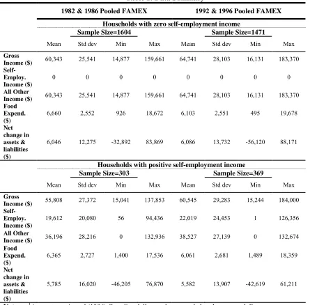
Table 1 provides some summary statistics of the data. The top half of the table presents

statistics for households with zero self-employment income, while the bottom half of the table

presents statistics for households with positive self-employment income. The left column shows

13

Similar estimates to those reported above were obtained when food expenditures were restricted to include only expenditures on food consumed at home.

14

Net change in assets and liabilities includes total net change in assets (including cash held in banks, money owed to households, money deposited against future purchases, net contributions less withdrawals to Registered Retirement Savings Plans, financial assets, sales of personal property, real estate, and investments in unincorporated business or farms) less net change in debts (including loans with regular payments and other money owed).

15

statistics for the 1982/1986 pooled sample and the right column for 1992/1996. The two

household groups report comparable average incomes, changes in assets, and expenditures on

food in each of the two samples, but self-employed households have greater variability in their

assets in the 1982/1986 sample.

3.2. Implementation Details of the Nonparametric Estimator

Nonparametric estimation of equations (3) and (4) is achieved by employing the

locally-weighted least-squares procedure, using the Gaussian kernel, and adaptive bandwidth where the

initializing bandwidth was selected by cross-validation (Härdle and Marron 1990). Equation (3),

the inverse Engel curve, is estimated at every point in the data but assigns a weight of zero to

households with positive self-employment income in the estimation process. The reporting

function given by equation (4) is estimated only for those households which report positive

self-employment income (y_{SE h,} >0).

3.3. Results

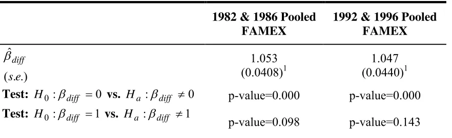
As outlined above, it is possible to test the significance of the A_h term in equation (3a).

The results of this test are outlined in Table 2. As before, the results for 1982/1986 are in the

column on the right and 1992/1996 are presented in the left-hand column. The parameter

estimates for _diff , noted in the first row, are very close to unity in value. In both cases, the null

hypothesis that _diff 0 is rejected with p-values of essentially zero, as is noted in the second

row of the table. The results for testing the null hypothesis that _diff =1 are shown in the third

1% or 5% significance levels but would be rejected at a 10% significant level. For the

1992/1996 pooled dataset, the null hypothesis that _diff 1 is not rejected at any conventional

significance level. Given the test results and the fact that the estimates for _diff are

economically no different from unity, it is concluded that the A term should be included in the

analysis as outlined above and proceed accordingly.

Figure 2 presents graphs of the inverse food Engel curve, estimated from equation (3a).

Recall from above that equation (3a) can be consistently estimated on the sample of households

that report zero self-employment income and provides an estimate of true household income for

all households. The graph on the left is for the 1982/1986 pooled sample while the graph on the

right is for 1992/1996. Reported food expenditure is plotted on the horizontal axis and gross

household income, less changes in assets, is plotted on the vertical axis. For both samples, the

inverse food Engel curve appears linear over most food expenditures, but takes on some

curvature at higher levels of food expenditures, notably where the data becomes sparse.16 Figure 3 presents graphs of the nonparametrically estimated reporting function that were

obtained using equation (4). Again, the graph on the left is for the 1982/1986 pooled sample

while the graph on the right is for 1992/1996. Estimated true self-employment income is plotted

on the vertical axis and reported self-employment income is plotted on the horizontal axis. Both

axes use the log scale. Also shown are 90% bootstrapped confidence intervals obtained using the

“wild” bootstrap procedure (Wu 1986) which allows for heteroskedastic errors. The forty-five

degree line in the figures shows reported self-employment income. When the plot of estimated

16

true self-employment income is above the forty-five degree line, a household is under-reporting

their self-employment income. Each graph also presents three vertical lines, which represent the

tenth, fiftieth, and ninetieth percentiles of the data. This information is presented to provide the

reader with detail regarding the density of the data and its relation to the estimation of the

reporting function.

The graphs in Figure 3 show that the reporting function appears to be nonlinear. For the

1982/1986 pooled sample, estimated true employment income is above reported

self-employment income for households with less than almost $40,000 in reported self-self-employment

income, but under-reporting decreases as reported self-employment income approaches

approximately $40,000. For the 1992/1996 pooled sample, estimated true self-employment

income is above reported self-employment income for households with less than just over

$40,000 in reported employment income, but under-reporting decreases as reported

self-employment income increases beyond approximately $40,000. While this result may appear to

be counter-intuitive, it supports the primary result of the model of tax compliance proposed by

Reinganum and Wilde (1985, 1986).

Beyond the approximate $40,000 threshold amount in both samples, the results indicate

that households over-report self-employment income. It should be noted that the estimated

number of married households that over-report is small in percentage terms. There are two

possible explanations for the over-reporting finding. First, this particular result could be driven,

at least in part, by data sparsity and a breakdown in the nonparametric procedures. In both

pooled samples, the data are sparse beyond $40,000. In the 1982/1986 pooled sample, the

ninetieth percentile occurs at approximately $46,800 ($55,000 in the 1992/1996 pooled sample).

self-employment income falls below reported self-self-employment income. Second, some self-employed

households may over-report their income due to a misinterpretation of tax laws, to avoid a tax

audit, to secure financing, and/or to exploit various tax deductions, credits and loopholes in an

effort to reduce their tax bill. This is an issue that has not received a lot of attention in the tax

evasion literature to date and the parametric restriction imposed on the Expenditure-Based

Method previously masked this possible behaviour. It should be noted that Rice (1992), using

the U.S. Internal Revenue Service’s (IRS) Tax Compliance Measurement Program (TCMP) data,

found that about 6% of firms overstate their taxable income to some extent, providing some

support for this hypothesis.

As mentioned above, it is possible to test whether or not the reporting function, equation

(4), is linear, as assumed previously in the literature. Table 3 summarizes the results of the test

of null hypothesis, that the reporting function takes the form of equation (1), against the

alternative, that the reporting function takes the nonparametric specification of equation (4). The

results for the 1982/1986 pooled dataset are noted in the first column. The value of the test

statistic is noted in the first row and the associated p-value is reported in the second row. A

value for the test statistic of 1.306 is obtained with an associated p-value of 0.096; hence, the null

hypothesis,H₀: y_{SE h}* _, y_{SE h,} , is rejected in favour of the alternative, H_a:y_{SE h}* _,  f y( _{SE h,} ),

at the 10% significance level. For the 1992/1996 pooled dataset, the results of which are

reported in the column on the left of Table 3, a value for the test statistic of 2.863 is obtained,

noted in the first row, with an associated p-value of essentially zero, shown in the second row.

Therefore, the null hypothesis is rejected at all of the usual significance levels. However, some

caution should be exercised in interpreting these results since this test statistic is known to suffer

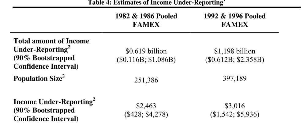
Table 4 reports household population estimates of income under-reporting by the

Canadian self-employed for 1982/1986, presented in the column on the left, and 1992/1996 in

the column on the right. The total amount of income under-reporting is found by subtracting

reported self-employment income from estimated household true self-employment income and

summing up over households. The first row of table 4 shows the population estimates for total

income reporting, obtained by using the FAMEX survey weights. Total income

under-reporting almost doubled between the 1980’s and the 1990’s, amounting to just over $0.619

billion in the 1982/1986 pooled sample and increasing to approximately $1.198 billion in the

1992/1986 pooled sample. The associated 90% bootstrapped confidence intervals are noted in

the parenthesis. There are two things to note with respect to the reported confidence intervals.

First, for both samples, the confidence intervals indicate that total income under-reporting was

statistically significantly greater than zero. Second, the overlapping of the confidence intervals

suggests that total income under-reporting in 1992/1996 was not statistically significantly

different from total income under-reporting in 1982/1986. Further statistical tests confirm that

the difference is not statistically significant.

As the number of self-employed households increased between the two pooled samples,

as shown in the second row of table 4, it could be that the increase in total income

under-reporting was simply due to the increase in self-employed households over the sample period,

rather than due to the implementation of the GST. In order to determine if there was a change in

the amount of income reporting per household, the average per household income

under-reporting is calculated.17 Despite the fact that the number of self-employed households increased

17

between these two pooled samples, there was an increase in the average amount of

self-employment income that went unreported. Income under-reporting per married household,

presented in the third row, amounted to $2,462.70 in the 1982/1986 pooled sample and

$3,015.71 in the 1992/1996 pooled sample. The 90% bootstrapped confidence intervals for these

per household amounts are presented in the final row of the table. Again, for both samples, the

confidence intervals indicate that average income under-reporting is statistically significant, but

the results are not statistically different from each other. That is, the results do not support the

notion that the GST increased income under-reporting by married households with

self-employment income. The results also do not support the claim that the GST would decrease tax

evasion.

3.4. Limitations

The results presented above call into question many of the assumptions made in the

parametric approach of the Expenditure-Based Method. That said, some caution needs to be

exercised in interpreting these specific results, as the reliability of the estimate depends on the

quality of the data. There are some notable features of the FAMEX that may bias the results

reported in this paper.

First, by using survey data, only those households that elected to take part in the survey

can be studied. Households that are heavily involved in underground activity, particularly those

households that are involved in illegal activity (for example, drug trafficking, human smuggling,

and prostitution), are unlikely to participate in the survey or may elect to modify their reported

Second, unlike household income and expenditure surveys conducted in other countries,

the FAMEX is a recall survey. That is, the data for the FAMEX is collected in March/April of a

given year, but covers expenditures for the previous year. It is possible that the expenditure data

used in the analysis may suffer from recall bias.18 In addition, data collectors make attempts to ensure that total expenditures are roughly equal to total income. In particular, income must

balance expenditures to within 10% and records where expenditures exceed all sources of

income by 20% or more are rejected. As a result, it is reasonable to assume that the estimates

obtained for the underground economy using this method will be a lower bound estimate. The

response rate for the FAMEX averages around 70%.

Third, income reported in the FAMEX may not be the same as income reported to the tax

authority by households. Households are not required to produce any proof of income and there

is no note in the FAMEX if the interviewer reviewed any such documents. To the extent that

income reported in the FAMEX differs from that reported to the tax authority, the results

outlined in this paper will be biased but it is unclear in which direction the results will be biased.

Finally, the unit of analysis, ideally, would be individuals, as it would avoid assuming

households act as single decision makers and because in Canada, taxes are assessed on the

individual rather than the household. In the FAMEX, however, expenditures are only surveyed

at the household level and there are insufficient observations to conduct the analysis on single

adult households. Additionally, as the FAMEX does not contain information regarding after-tax

income by income source19, the application was conducted using gross income. After-tax

18

Ahmed et al. (2005) compare income and food expenditure information collected in a diary based survey (FOODEX) to those collect in a recall based survey (FAMEX) and find little difference.

19

income is more desirable in this analysis as households are more likely to base their expenditures

on after-tax income. Further, as previously mentioned, income tax in Canada is assessed on the

individual rather than on the household. As a result, households with similar gross incomes, may

not have comparable net income and hence may not have comparable expenditures, which would

lead to a biased estimate of true gross income in the first step of the approach.

This analysis was also conducted on married households, living in both rural and urban

areas. Limiting the analysis to households living only in urban areas, resulted in insufficient

observations. It is extremely likely that households in urban and rural environments, have

different levels of food expenditures at similar income levels for reasons that are unassociated

with income under-reporting. For example, households in rural environments may be more

likely to: grow food for consumption in a household garden; face reduced food prices due to the

presence of local producers and suppliers; and engage in the trade of goods and services for food

products. To the extent that this is true, food expenditures for rural households with no

employment income will act as a poor counterfactual for urban households with positive

self-employment income and vice versa.

Caution must also be exercised in interpreting and comparing the results presented here

to those obtained by alternate methods. The results presented here, income under-reporting by

married households with self-employment income, should not be interpreted as representing a

measure of the total underground economy. Households with self-employment income but with

different demographic characteristics (e.g. households with children, single person households

etc.) may engage in income under-reporting at different rates than married households.

Additionally, income under-reporting by the self-employed, represents only a portion of

underground activity. Finally, the method presented in this paper, estimates income that is not

reported to tax authorities, which is quite distinct from measuring production or income that is

missed by the statistical offices when they calculate the value of the national product. Many

methods employed in estimating underground activity use the latter calculation. Giles and Tedds

(2002), updated by Tedds (2005), provide a summary of the available Canadian estimates of

underground activity, arranged according to methodology and calculation employed, should

additional, independent comparisons be desired.

4. CONCLUSION

This paper proposes a nonparametric approach for estimating income under-reporting by

households with self-employment income. The use of nonparametric methods is shown to have

several advantages over previous parametric approaches. First, it enables the reporting function

to vary across income levels and household characteristics. Second, it provided the ability to

test, and find evidence against, the previously held hypothesis that the reporting function takes

the linear form. Third, the framework allowed for an alternative approach to addressing the issue

of permanent income. A further advantage of this method is the ease in which population

estimates can be generated. In particular, the total amount of unreported income in the

population could be obtained directly, whereas previous studies could only extrapolate this

information by using national accounts data. Overall, the approach outlined in this paper calls

into question many of the assumptions made in the parametric applications of the

Expenditure-Based Method.

The approach outlined in this paper is illustrated by estimating the effect of the Canadian

self-employment income. The results indicate that income under-reporting by married households

with self-employment income neither increased nor decreased following the implementation of

the GST. The results indicate that income under-reporting increased, in real (1996) dollar terms,

from $2,462.70 per household in the 1980’s to $3,015.71 per household in the 1990’s, following

the implementation of the GST, but that this difference is not statistically significant. Caution

needs to be exercised in interpreting these specific results, as the reliability of the estimate

depends on the quality of the data and on the various assumptions made. Evidence is provided

that supports the notion that the obtained estimates of income under-reporting reported in this

paper are lower bound estimates.

The analysis presented in this paper indicates that further work is required in refining this

method to improve consistency with available data and knowledge concerning participation in

the underground economy. In particular, redefining the base group is warranted, as is exploring

a relaxation of the assumption that requires the marginal propensity to consume out of

unreported income to equal the marginal propensity to consume out of reported income. It may

also be worthwhile to consider alternative forms of the reporting function. Finally, several

shortcomings related to the use of the FAMEX were described in this paper, shortcomings that

are shared by comparable data sets for other countries. The most important of these is that

income reported in the FAMEX may not be the same as income reported to the tax authority by

households because households are not required to produce any proof of income. Tax filer data,

on the other hand, would have exact information regarding income and, hence, would provide

more accurate estimates of income under-reporting. Unfortunately, tax filer data does not

contain detailed information regarding expenditures. It does, however, contain information

may be possible to use this information and the method outlined in this paper to obtain more

REFERENCES

Ahmed, Naeem, Matthew Brzozowski and Thomas F. Crossley (2005), “Measurement Errors in Recall Food Expenditure Data,” Working Paper, Department of Economics, McMaster University, WP 2004-16.

Banks, J., Blundell, R., and Lewbel A. (1997), “Quadratic Engel Curves and Consumer Demand,”. Review of Economics and Statistics, 4, 527-538.

Blundell, R., Duncan A., and Pendakur K. (1998), “Semiparametric Estimation and Consumer Demand,”Journal of Applied Econometrics, 13, 435-461.

Browning, M. and Thomas, I. (1999), “Prices for the FAMEX: Methods and Sources,” Working Paper, Department of Economics, McMaster University.

Dilnot, A.W. and Morris, C.N. (1981), “What do We Know About the Black Economy?”Fiscal Studies, 2, 58-73.

Feige, E.L. (1979), “How Big is the Irregular Economy?”Challenge, 22, 5-13.

Frey, B.S. and Weck-Hanneman, H. (1984), “The Hidden Economy as an Unobserved Variable,”

European Economic Review, 26, 33-53.

Giles, D.E.A. and Tedds, L.M. (2002) Taxes and the Canadian Hidden Economy, Toronto: Canadian Tax Foundation.

Gutmann, P.M. (1977), “The Subterranean Economy,”Financial Analysts Journal, 34, 24-27.

Härdle, W. and Marron, J.S. (1990), “Semiparametric comparison of Regression Curves,”Annals of Statistics, 18, 63-89.

Hill, R. and Kabir, M.. (1996), “Tax Rates, the Tax Mix, and the Growth of the Underground Economy in Canada: What Can We Infer,”Canadian Tax Journal, 44, 1552-1583.

Lyssiotou, P., Pashardes, P. and Stengos, T. (2004), “Estimates of the Black Economy Based on Consumer Demand Approaches,”Economic Journal, 114, 622-639.

Mirus, R. and Smith, R.S. (1997), “Self-Employment, Tax Evasion, and the Underground Economy: Micro-Based Estimates for Canada,” Working Paper, International Tax Program, Harvard Law School.

Pissarides, C.A. and Weber, G. (1989), “An Expenditure-based Estimate of Britain’s Black Economy,”Journal of Public Economics, 39, 17-32.

Reinganum, Jennifer F. and Louis L. Wilde (1985), “Income Tax Compliance in a Principal-Agent Framework,” Journal of Public Economics, 26, 1-18.

______. (1986), “Equilibrium Verification and Reporting Policies in Model of Tax Compliance,” International Economic Review, 27, 739-760.

Rice, E.M. (1992), “The Corporate Tax Gap: Evidence on Tax Compliance by Small Corporations,” in Why People Pay Taxes: Tax Compliance and Enforcement, ed. Joel Slemrod, 125-166, Ann Arbor: The University of Michigan Press.

Schuetze, H.J. (2002), “Profiles of Tax Noncompliance Among the Self-Employed in Canada, 1969-1992,”Canadian Public Policy, XXVIII, 219-237.

Smith, S. with Pissarides, C.A. and Weber, G. (1986), “Evidence from Survey Discrepancies,” in

Britain’s Shadow Economy, ed. Stephen Smith, 137-153, Oxford: Clarendon Press.

Spiro, P.S. (1993), “Evidence of a Post-GST Increase in the Underground Economy,” Canadian Tax Journal, 41, 247-258.

Tanzi, V. (1980), “The Underground Economy in the United States: Estimates and Implications,”

Banco Nazionale del Lavoro, 135, 427-453.

Tedds, L.M. (2005), “The Underground Economy in Canada,” in Size, Causes and Consequences of the Underground Economy, ed. by Chris Bajada and Friedrich Schneider. Aldershot: Ashgate Publishing (forthcoming).

Thomas, J. (1999), “Quantifying the Black Economy: Measurement without Theory Yet Again,”

Economic Journal, 109, F381-F337.

Wu, C.F.J. (1986), “Jackknife, Bootstrap, and Other Resampling Methods in Regression Analysis,”Annals of Statistics, 14, 1261-1350.

Yatchew, A. (1998), “Nonparametric Regression Techniques in Economics,” Journal of Economic Literature, 36, 669-721.

TABLES

Table 1: Data Summary1

1982 & 1986 Pooled FAMEX 1992 & 1996 Pooled FAMEX

Households with zero self-employment income

Sample Size=1604 Sample Size=1471

Mean Std dev Min Max Mean Std dev Min Max

Gross

Income ($) 60,343 25,541 14,877 159,661 64,741 28,103 16,131 183,370

Self-Employ. Income ($)

0 0 0 0 0 0 0 0

All Other

Income ($) 60,343 25,541 14,877 159,661 64,741 28,103 16,131 183,370

Food Expend. ($)

6,660 2,552 926 18,672 6,103 2,551 495 19,678

Net change in assets & liabilities ($)

6,046 12,275 -32,892 83,869 6,086 13,732 -56,120 88,171

Households with positive self-employment income

Sample Size=303 Sample Size=369

Mean Std dev Min Max Mean Std dev Min Max

Gross

Income ($) 55,808 27,372 15,041 137,853 60,545 29,283 15,244 184,000

Self-Employ. Income ($)

19,612 20,080 56 94,436 22,019 24,453 1 126,356

All Other

Income ($) 36,196 28,216 0 132,936 38,527 27,139 0 132,674

Food Expend. ($)

6,365 2,727 1,400 17,536 6,061 2,681 1,489 18,359

Net change in assets & liabilities ($)

5,785 16,020 -46,205 76,870 5,582 13,907 -42,619 61,211

Table 2: Testing the Significance of A_h

1982 & 1986 Pooled FAMEX

1992 & 1996 Pooled FAMEX

.) . (

ˆ

e s

diff

 _1.053

(0.0408)1

1.047 (0.0440)1 Test: H₀:_diff 0 vs. H_a :_diff 0 p-value=0.000 p-value=0.000 Test: H₀:_diff 1 vs. H_a :_diff 1

p-value=0.098 p-value=0.143

Notes: 1Standard errors corrected for autocorrelation as discussed in the text.

Table 3: Testing Linearity of the Reporting Function

Test: H₀ : y*_{SE h,} y_{SE h,} vs. H_a:y*_{SE h,}  f y( _{SE h,} )

1982 & 1986 Pooled FAMEX 1992 & 1996 Pooled FAMEX

V

p-value

1.306

0.096

2.863

Table 4: Estimates of Income Under-Reporting1 1982 & 1986 Pooled

FAMEX

1992 & 1996 Pooled FAMEX

Total amount of Income Under-Reporting2

(90% Bootstrapped Confidence Interval)

$0.619 billion ($0.116B; $1.086B)

$1,198 billion ($0.612B; $2.358B)

Population Size2 _251,386 397,189

Income Under-Reporting2 (90% Bootstrapped Confidence Interval)

$2,463 ($428; $4,278)

$3,016 ($1,542; $5,936)

Notes 1Amounts are in real (1996) Canadian dollars and are rounded to the nearest dollar.

2

Calculated for married households without dependent children present in the hosuehold that report positive self-employment income using the survey

FIGURES

Figure 1: Income Under-reporting in the Single Equation Expenditure-Based Method

Log of

Expenditures Self-Employed

Households

Employee Households

Y Y*

E*

F

igu

re

2:

I

n

ve

rs

e F

ood

E

n

ge

l C

u

rve

38