Productivity shocks and Optimal Monetary Policy in a Unionized Labor Market Economy

Munich Personal RePEc Archive

Productivity shocks and Optimal

Monetary Policy in a Unionized Labor

Market Economy

Mattesini, Fabrizio and Rossi, Lorenza

Università di Roma "Tor Vergata"

June 2006

Online at

https://mpra.ub.uni-muenchen.de/2828/

Productivity shocks and Optimal Monetary

Policy in a Unionized Labor Market Economy

Fabrizio Mattesini

Università di Roma ”Tor Vergata”

Via Columbia 2, 00133 Roma, It

Lorenza Rossi

Istituto di Economia e …nanza

Università Cattolica del Sacro Cuore

Via Necchi, 5 - 20123 - Milano, It

EABCN

April 2007

Abstract

and a trade-o¤ between in‡ation stabilization and the output stabi-lization arises. In particular, a productivity shock has a negative e¤ect on in‡ation, while a reservation-wage shock has an e¤ect of the same size but with the opposite sign. We derive a welfare-based objective function for the Central Bank as a second order Taylor approxima-tion of the expected utility of the economy’s representative household, and we analyze optimal monetary policy under discretion and under commitment. Under discretion a negative productivity shock and a positive exogenous wage shock will require an increase in the nomi-nal interest rate. An operationomi-nal instrument rule, in this case, will satisfy the Taylor principle, but will also require that the nominal in-terest rate does not necessarily respond one to one to an increase in the interest rate that supports the e¢cient equilibrium. The results of the model are consistent with a well known empirical regularity in macroeconomics, i.e. that employment volatility is relatively larger than real wage volatility.

1

Introduction

In the last ten years, the Dynamic Stochastic New Keynesian (henceforth, DSNK) model has emerged as an important paradigm in macroeconomics and as a useful framework for the study of monetary policy. Most of the models proposed so far along this line of research, however, are based on the standard competitive model and completely ignore the role that trade unions play in determining wages and employment conditions in many countries. If this is probably an acceptable (although very strong) simpli…cation for coun-tries, like the U.S., where in the year 2002, only about 15% of workers were covered by collective contract agreements, it becomes instead problematic for other countries such as France, Italy or Sweden where the percentage of workers covered by collective contracts is above 84%.1 _{Given that wage}

bar-gaining may introduce signi…cant distortions in the functioning of a modern economy and have an impact on its behavior at the aggregate level, the study of unionized labor markets and of the consequences of these markets for mon-etary policy becomes of crucial importance if one wants to understand the functioning of many important economies around the world.

The purpose of this paper is to propose a model where wages are the result of a contractual process between unions and …rms and where, at the same time, the movements of the rate of unemployment are explicitly accounted for. In order to evaluate movements of labor along the extensive margin, we assume, as in Hansen [22] and Rogerson and Wright [30], that labor supply is

1_{More precisely, the number of persons covered by collective agreeements over total}

indivisible and that workers face a positive probability to remain unemployed. As in Ma¤ezzoli [25] and Zanetti [38], we assume that wages are set by unions according to the popular monopoly-union model introduced by Dunlop [12] and Oswald [27]. This paper, therefore, contributes to a literature which has recently tried to improve on the ”standard” DSNK model by focusing on the behavior of the labor market. Models characterized by labor market frictions and price staggering, where labor is allowed to move not only along the intensive margin but also the extensive margin, have been proposed, among others, by Chéron and Langot [7], Walsh [34] [35], Trigari [32], [33], Moyen and Sahuc [26] and Andres et al. [2]. More recently Christo¤el and Linzert [9] and Blanchard and Galì [4] [5] have proposed models characterized not only by labor market frictions and staggered prices, but also by real wage rigidities. Blanchard and Galì [4] show that, if real wages are assumed to adjust slowly, what they de…ne as the ”divine coincidence” does not hold any more: for a central bank pursuing, as a policy objective, the level of output that would prevail under ‡exible prices is not equivalent to pursuing the e¢cient level of output, in which case a trade-o¤ between in‡ation stabilization and output gap stabilization arises. Blanchard and Galì [5] analyze a model where labor market frictions are not simply assumed but explicitly modelled and show that a policy trade-o¤ does not only pertain to the output gap, but also to the rate of unemployment.

introduce unemployment in an alternative simple and tractable way which allows us to establish an inverse relationship between unemployment and the output gap and we focus on the consequences of union behavior for the response of the economy to exogenous shocks. The model is capable of producing a series of interesting results.

First, it shows that productivity shocks give rise to a signi…cant policy trade-o¤ between stabilizing in‡ation and stabilizing unemployment, and in this respect it provides a way to overcome an important shortcoming of the DSNK model, i.e. its inability to account for the signi…cant challenges that exogenous changes in technology represent for monetary policy in the real world. According to the ”standard” DSNK model, in fact, an optimal mon-etary policy that stabilizes output around its ‡exible price equilibrium, also produces zero in‡ation,2 _{so that stabilizing in‡ation implies automatically}

an optimal response to a productivity shocks. This, however, not only is at odds with the historical accounts3 _{and the widespread perception of}

…-nancial markets, but there is also some recent empirical evidence indicating that, in most countries, central banks have actively responded to technology shocks, increasing or decreasing the nominal interest rate.4 _{What is}

interest-2_{This is shown quite clearly, for example, by Galì, Lopez Salido and Valles [16].}

3_{In this respect the debate on the Fed’s monetary policy during governor Greenspan}

tenure is quite instructive. There is a lot of anectodical evidence that the Fed has spent large e¤orts in understanding the increase in productivity growth that has characterized the American economy since the mid 1990s. The success of monetary policy in this period has been attributed by important commentators (Woodward 2000) to the ability of the Fed to respond to exogenous technological progress.

4_{Galì et al. [15], analyzing a 4 variable SVAR model where thechnology shocks were}

ing, in our model, is that this result is not the consequence of some kind of exogenous real wage inertia, as in Blanchard and Galì [4], but is simply the consequence of unions’ monopoly power in the labor market. In our economy, in fact, a productivity slowdown, i.e. a negative productivity shock tends to lower e¢cient output but, since unions will keep real wages constant, the level of output that would prevail under price ‡exibility, that we de…ne as ”natural” output, decreases even more, so that the di¤erence between e¢-cient output and ”natural” output increases. Since in sticky price models in‡ation depends on marginal costs and, in turn, marginal costs depend on the di¤erence between ”natural” output and actual output, then a Phillips curve, correctly de…ned as depending on the gap between e¢cient output and actual output, will depend on productivity shocks, and a trade-o¤ between in‡ation stabilization and output gap stabilization arises.

Second, we show that a policy trade-o¤ for the central bank arises not only in response to technology shocks, but also in response to exogenous wage push shocks. If the unions’ reservation wage is subject to exogenous changes, and these changes tend to be persistent over time, then a welfare maximiz-ing central bank must again face the problem of whether to accommodate these shocks with a easier monetary policy. Our model therefore provides a convenient framework to address important normative issues such as, for example, the optimal behavior of central banks in periods characterized by

labor market turmoil and exogenous wage shocks.

Third, we derive the objective function of the central bank as a second order Taylor approximation of the expected utility of the representative household and we show that, when the economy is hit by technology and ex-ogenous wage shocks, monetary policy presents some interesting peculiarities relative to the standard case. We …rst consider the problem of a central bank that cannot commit to future policy actions. In this case optimal monetary policy requires a decrease (increase) in the interest rate following a positive (negative) productivity shock and an increase in the interest rate following a reservation wage shock. An optimal instrument rule that implements such policy can be expressed as an interest rate reacting to the expected rate of in‡ation and to the natural rate of interest. In this model monetary policy satis…es the Taylor principle, i.e. the nominal interest rate must be raised more than proportionally with respect to the expected rate of in‡ation. Dif-ferently from the standard model, however, the nominal interest rate must not increase one to one with the natural rate of interest. If the persistence of the technological shock is greater than the persistence of the reservation wage shock the nominal interest will increase less than proportionately to an increase in the rate of interest that supports the e¢cient equilibrium.

real wage and in the rate of unemployment; a productivity shock, instead, will induce a movement in the rate of unemployment, but not in the real wage. An economy frequently hit by exogenous changes in technology will show, therefore, a strong variability in the rate of unemployment without experiencing, at the same time, signi…cant movements in the real wage.5

The model is calibrated not only under the optimal rule, but also un-der other simpler operational rules. We show that an optimal discretionary monetary policy requires a reaction to in‡ation which is less aggressive than the one required by strict in‡ation targeting, but more aggressive than the one required by a policy of full employment stabilization. We also show that an optimal monetary policy may be replicated by a simple Taylor rule. A rule that is capable to deliver impulse response functions similar to the ones implied by the optimal rule, however, implies that the reaction to in‡ation is quite high relative to the most popular estimates, and a smaller reaction to the output gap.

The paper is organized as follows. In Section 2 we start by introducing indivisible labor in a standard DSNK model with Walrasian labor markets. In Section 3 we develop the unionized labor market model. In Section 4 we study optimal monetary policy and, …nally, in Section 4 we calibrate the model under the optimal rule and some simpler policy rules.

5_{Also Gertler and Trigari [19] propose a model where wages and unemployment move}

2

A model with Indivisible Labor and

Wal-rasian Labor Market

2.1

The Representative Household

We consider an economy populated by many identical, in…nitely lived worker-households each of measure zero. Households demand a Dixit, Stiglitz [11] composite consumption bundle produced by a continuum of monopolistically competitive …rms. In each period households sell labor services to the …rms. As in Hansen [22], Rogerson [30] and Rogerson and Wright [31], for each household the alternative is between working a …xed number of hours and not working at all. We assume that agents enter employment lotteries, i.e. sign, with a …rm, a contract that commits them to work a …xed number of hours, that we normalize to one, with probability Nt: The contract itself is

being traded, so a household gets paid whether it works or not which implies that the …rm is providing complete unemployment insurance to the workers. Since all households are identical, all will choose the same contract, i.e. the same Nt: However, although households are ex-ante identical, they will

dif-fer ex-post depending on the outcome of the lottery: a fraction Nt of the

continuum of households will work and the rest 1 Nt remains unemployed.

The allocation of individuals to work or leisure is determined completely at random by a lottery, and lottery outcomes are independent over time. Before the lottery draw, the expected intratemporal utility function is:

1

1 Nt[C0;t (0)]

1

+ 1

1 (1 Nt) [C1;t (1)]

1

where C0;t is the consumption level of employed individuals, C1;t is the

con-sumption of unemployed individuals, Nt is the ex-ante probability of being

employed and ( ) is the utility of leisure. Since the utility of leisure of em-ployed individuals (0) and the utility of leisure of unemployed individuals

(1) are positive constants, we assume (0) = 0 and (1) = 1:As in King and Rebelo [21], we assume 0 < 1:

If asset market are complete, households can insure themselves against the risk of being unemployed. Under perfect risk sharing we have:

C_0;t 1₀ =C_1;t 1₁ (2)

which implies that the marginal utilities of consumption are equal for em-ployed and unemem-ployed individuals. De…ning the average consumption level as:

Ct=NtC0;t+ (1 Nt)C1;t

and given (2), equation (1) can be rewritten as:

1

1 C

1

t

h

Nt

1

0 + (1 Nt)

1 1

i

: (3)

This allows us to write the life-time expected intertemporal utility function of a representative household as:

Ut =Et

1

X

=t

t 1

1 [Ct (Nt)]

1

; (4)

function

(Nt) =

h

Nt

1

0 + (1 Nt)

1 1

i₁

can be interpreted as the disutility of employment for the representative household. The elasticity of (Nt) with respect to its argument is given

by = N(Nt)

(Nt) N < 0. The ‡ow budget constraint of the representative household is given by:

PtCt+Pt 1Bt+1 WtNt+Bt+ t Tt (5)

where Pt is the corresponding consumption price index (CPI) andWt is the

wage rate. Notice that here a worker is paid according to the probability that it works, not according to the work it does; in other words, the …rm is automatically providing full employment insurance to the households. The purchase of consumption goods, Ct; is …nanced by labor income, pro…t

in-come t; and a lump-sum transfers Tt from the Government. Households

have access to a …nancial market, where nominal bonds are exchanged. We denote byBt the quantity of nominally riskless one period bonds carried over

from period t 1; and paying one unit of the numéraire in period t. The maximization of (4) subject to (5) gives the following::

1 = RtEt

"

Ct+1

Ct

(Nt)

(Nt+1) 1

Pt Pt+1

#

(6)

Wt Pt

= Ct N

(Nt)

(Nt)

(7)

us the supply of labor of the representative household.

2.2

The Representative Finished Goods-Producing Firm

The representative …nished goods-producing …rm uses Yt(j) units of each

intermediate good j 2 [0;1] purchased at a nominal price Pt(j) to produce Yt units of the …nished good with the constant returns to scale technology:

Yt =

Z 1

0

Yt(j)

1

dj

1

(8)

where is the elasticity of substitution across intermediate goods. Pro…t maximization yields the following set of demands for intermediate goods:

Yt(j) =

Pt(j) Pt

Yt (9)

Perfect competition and free entry drives the …nished good-producing …rms’ pro…ts to zero, so that from the zero pro…t condition we obtain:

Pt=

Z 1

0

Pt(j)1

1 1

: (10)

which de…nes the aggregate price index of our economy.

2.3

The Representative intermediate Goods-Producing

Firm

of labor from the representative household and produce Yt(j) units of the

intermediate good using the following technology:

Yt(j) = AtNt(j) (11)

where At is an exogenous productivity shock. We assume that the lnAt at follows follows the autoregressive process

at= aat 1+ ^at (12)

where a<1and^atis a normally distributed serially uncorrelated innovation

with zero mean and standard deviation a.

Before choosing the price of its goods, a …rm chooses the level ofNt(j)which

minimizes its costs, solving the following costs minimization problem:

min fNtg

T Ct = (1 )WtNt(j)

subject to (11), where represents an employment subsidy to the …rm6_{. The}

…rst order condition with respect to Nt(j) is given by:

(1 )Wt

Pt

=M Ct(j)

Yt(j) Nt(j)

; (13)

where M Ct(j) represents …rm’s j marginal costs. De…ning aggregate

mar-6_{We assume that the subsidy is covered by a lump sum tax in that the Government}

ginal costs as:

M Ct=

(1 )Wt Pt

Nt Yt

: (14)

2.4

Market clearing

Equilibrium in the goods market of sector j requires that the production of the …nal good be allocated to expenditure, as follows:

Yt(j) =Ct(j) (15)

considering (8) then

Yt =Ct (16)

which represents the economy resource constraint.

Since the net supply of bonds, in equilibrium is zero, equilibrium in the bonds market, instead, implies

Bt= 0: (17)

Labor market clearing implies

Nt=

Z 1

0

Nt(j)dj (18)

given equation (9), (11) and (18) the aggregate production function can be expressed as

where

Dt=

"Z 1

0

Pt(j) Pt

dj

#

(20)

is a measure of price dispersion.

De…ning as X the steady state value of a generic variable Xt and by xt = lnXt lnX the log-deviation of the variable from its steady state

value, then a linear …rst order approximation of the resource constrained around the steady state is given by:

yt=ct (21)

Given that in a neighborhood of a symmetric equilibrium and up to a …rst order approximation Dt'1; log-linearizing equation (19) we obtain,

yt =at+ nt: (22)

2.5

The First Best Level of Output

The e¢cient level of output can be obtained by solving the problem of a benevolent planner that maximizes the intertemporal utility of the repre-sentative household, subject to the resource constraint and the production function. This problem is analyzed in the Appendix A1, where we show that the e¢cient supply of labor, in our economy, is given by:

N(Nt)

(Nt)

Log-linearizing (23), and considering (22), we obtain7

ytEf f =at: (24)

2.6

The Flexible Price Equilibrium and the Natural

Output

Equilibrium in the labor market is obtained by equating (7) and (14). Sub-stituting (16), this implies

Yt N

(Nt)

(Nt)

= 1

(1 ) M Ct

Yt Nt

(25)

Under ‡exible prices, all …rms set their prices equal to a constant markup over marginal cost. Assuming that …rms mark-up, P

t is constant, under

the ‡exible price-equilibrium …rms real marginal costs are constant at their steady state level and therefore given by:

M Ct=

1

1 + P: (26)

Considering now the log-linearization of (25) we obtain8_,

mct = 1 + N

(N) (N) N

N N(N)N2

(N) nt (27)

Considering that mct = 0;then nt = 0 and, from the aggregate production

7_{See appendix A2.}

function, we have that under the ‡exible price equilibrium:

ytf =at: (28)

Taking the di¤erence between the log-linearized ‡exible and e¢cient output we obtain:

y_tEf f yf_t = 0 (29)

As in the standard DSNK model, when labor market is frictionless the dif-ference between the e¢cient output (its …rst best) coincides with its ‡exible price equilibrium level (its second best) that we have de…ned as the natural level of output.9 _{In other words, what Blanchard and Galì [4] call ”the}

di-vine coincidence” will hold, since any policy that stabilizes output around its natural level, will stabilize it also around its e¢cient level. Notice that, in this model we have left the subsidy as parametric in order to show that the divine coincidence holds for any possible value of the subsidy. As in the standard case, also in this model an optimal subsidy could be set in order to eliminate the constant distortion induced by monopolistic competition.

9_{Our result is equivalent to the one of Blanchard Galì, where they consider (log) real}

2.7

The Phillips Curve

Firms choose Pt(j) in a staggered price setting à la Calvo-Yun [6]. In the

appendix A4 we show that, in our decreasing return to scale economy, the solution of the …rm’s problem is given by:

t = Et t+1+ mct (30)

where = (1 )(1 ) _{+ (1 )} and is the probability with which …rms reset prices.

Given (22), (27) and (28), marginal costs can be rewritten in terms of the gap between actual and natural output,

mct = 1 + N

(N) (N) N

N N (N)N2

(N) yt y

f

t (31)

so that, equation (30) can be rewritten as,

t= Et t+1+ a 1 + N

(N) (N) N

N N(N)N2

(N) xt (32)

where a = (1 ')(1_' ' ) _{+ (1 )} and

xt=yt ytf (33)

3

A model with Indivisible Labor and a

Union-ized Labor Market

3.1

The Monopoly Union

As in the previous subsection the individual labor supply is indivisible. Each …rm is endowed with a pool of household from which it can hire. In fact, as in Ma¤ezzoli [25] and Zanetti [38], …rms hire workers from a pool composed of in…nitely many households so that the individual household member is again of measure zero. Since each household supplies its labor to only one …rm, which can be clearly identi…ed, workers try to extract some producer surplus by organizing themselves into a …rm-speci…c trade union. The economy is populated by decentralized trade unions, so that each intermediate goods-producing …rm negotiate with a single union i2(0;1);which is too small to in‡uence the outcome of the market. Unions negotiate the wage on behalf of their members.

welfare function10_:

Nt(i) Wt

Pt

+ (1 Nt(i)) Wr

t Pt

(34)

subject to …rms’ labor demand (13), where, Wr

t is the reservation wage.

The reservation wage, here, is not a direct aggregation of workers reserva-tion wages, but rather re‡ects the subjective evaluareserva-tion, by union leaders of workers’ disutility of labor.11 _{With equation (34) we assume that unions}

are risk neutral and maximize members average wage. We assume that the reservation wage follows a stochastic process. Denoting bywr

t the logarithm

of Wr

t we assume that:

wr

t = ww

r

t 1+ ^wrt (35)

where _w <1and wr

t is a normally distributed serially uncorrelated

innova-tion with zero mean and standard deviainnova-tion w.

The employment rate and the wage rate are determined in a non-cooperative dynamic game between the unions and the …rms. We restrict the attention to Markov strategies, so that in each period union and …rm solve a sequence of independent static games. Each union behaves as a Stackelberg leader and each …rm as a Stackelberg follower. Once the wage has been chosen, each …rm decides the employment rate along its labor demand function. Even if unions are large at the …rm level, they are small at the economy level, and therefore they take the aggregate wage as given. The ex-ante probability of

10_{The utility function above correspondes to the risk neutral analogue of the utilitarian}

utility function of Oswald [27]. Anderson and Devereux [1] and Pissarides [29] use a similar utility function.

11_{In principle the reservation wage could also represent any unemployment subsidy}

being employed is equal to the aggregate employment rate and the allocation of union members to work or leisure is completely random and independent over time.

From the …rst order conditions of the union’s maximization problem with respect to Wt(i)we have:

Wt(i) Pt

= 1W

r t Pt

: (36)

Since 1 _{> 1; this implies that the real wage rate is always set above the} reservation wage.

3.2

Households

Similarly to what happens in the previous model, also in this case households enter employment lotteries i.e. sign, with a …rm, a contract that commits them to work a …xed number of hours with probability Nt: By entering this

contract, which is being traded, a …rm provides complete unemployment insurance to the workers.12 _{As in the previous model, also in this model}

the marginal utility of consumption will be equalized across employed and unemployed workers, so that households can be aggregated in a representative household. Therefore, also in this model the life-time expected intertemporal utility function of a representative household can be written again as the problem of maximizing (4) subject to (??) and the ‡ow budget constraint (5).

12_{Alternatively, we could consider an institutional arrangement where the union o¤ers}

The model is quite similar to the previous model with walrasian labor markets, except for the fact that now households, in solving their problem, takeNtas given, since the supply of labor is determined by the maximization

problem of the monopoly union. The maximization of utility function subject to budget constraint gives the same Euler equation as in the Walrasian model, which is given by equation (6).

3.3

The Flexible Price Equilibrium and the Natural

Level of Output

Given that both intermediate goods and …nished goods producing …rm prob-lem are the same as in the previous probprob-lem, the aggregate labor demand function is again given by equation (14). Equating (14) and (36), we obtain:

1Wr t Pt

= 1

(1 ) M Ct

Yt Nt

: (37)

Since under ‡exible prices all …rms set their prices as a constant markup over marginal costs, which is given by equation (26), we can rewrite equation (37) as:

1Wr t Pt

= 1

(1 ) 1 1 + P

Yt Nt

(38)

Considering now the log-linearization of (37) we obtain the following expres-sion for real marginal costs

where wr

t is the logarithm of the real reservation wage. Solving (22) for nt

and substituting in (39), we get:

mct=wtr+

1

yt

1

at (40)

Considering that mct = 0; substituting in (40) and solving for yt we …nd

an expression for the ‡exible-price level of output, which we de…ne as the natural rate of output for our unionized economy:

ytf =

1

1 at 1 w

r

t (41)

Recalling now that the e¢cient level of output, for our economy with indivis-ible labor, is given by equation (24) we immediately see that the di¤erence between natural output and e¢cient output of the unionized economy is given by

ytEf f y f

t =

1 at+1 w

r

t: (42)

Unlike what happens in the walrasian model, this di¤erence is not constant, but is a function of the relevant shocks that hit the economy. In this model therefore, as in Blanchard and Galì [4] stabilizing the output gap - the di¤er-ence between actual and natural output - is not equivalent to stabilizing the

3.4

The Long Run Labor Market Equilibrium:

Opti-mal Subsidy

In this economy, when …rms can revise their price at each time, beside the distortion created by monopolistic competition and …rms’ markup we have a distortion created by the monopoly union wage setting. We assume that, at the steady state, the government uses the employment subsidy to the …rms , to bring steady state output to its e¢cient level, i.e. to the level at which

N(N)

(N) N = : (43)

Since in the unionized economy labor market equilibrium is given by:

1Wr

P =

1 (1 )

1 1 + P

Y

N; (44)

if the government sets a subsidy such that

Wr

P (1 ) (1 + P₎N

Y =

N(N)

(N) N (45)

which implies

= 1 + 1 1 + P

N(N)

(N) N

Y N

P

Wr : (46)

3.5

The IS-Curve

In order to obtain the IS curve we start by log-linearizing around the steady state the Euler equation (6). Considering that in steady state the optimal subsidy setting implies N(N)N

(N) = ; the log-linearized Euler equation is given by:

ct=Etfct+1g+

(1 )

Etf nt+1g

1

(^rt Etf t+1g): (47)

with r^t = rt %; where rt = lnRt and % = ln which is the steady state

interest rate all the variables without a subscript are taken at their steady state levels. Given the economy resource constraint (21) and the production function (22), the Euler equation (47) can be written as:

yt =Etfyt+1g (1 )Etf at+1g (rt Etf t+1g) (48)

which represents the IS equation of our simple economy.

Let us rede…ne, for the Unionized economy, the relevant output gap as the di¤erence between actual output and e¢cient output, i.e.,

xt=yt yEf ft : (49)

In this case the IS equation can be rewritten in terms of the output gap as,

xt =Etfxt+1g (rt Etf t+1g rte): (50)

where r^e

can be expressed as:

^

re

t = Etf at+1g= Et

n

yEf f_t+1 o= (1 a)at: (51)

Note that (50) expressed in terms of the gap between the actual and the e¢cient output relates the output gap to current and anticipated deviations of the real interest rate from its e¢cient counterpart.

3.6

The Phillips Curve

As in the Walrasian case, …rms choosePt(j)in a staggered price setting à la

Calvo-Yun [6] and the Phillips curve is again given by (30).

Given (39) and (41), marginal costs can be rewritten in terms of the gap between actual output and its natural level,

mct=

1

yt yft (52)

so that, equation (30) can now be rewritten as,

t= Et t+1+ a

1

yt ytf (53)

Given the relationship between e¢cient and natural output, (see eq. (42)), equation (53) can …nally be expressed as:

t= Et t+1+ a

1

xt at+ wtr (54)

We can now state:

Result 1. In a unionized labor market economy the ”divine coincidence”

does not hold, i.e., stabilizing in‡ation is not equivalent to stabilizing the

output gap de…ned as the deviation of output from the e¢cient output. A

positive (negative) productivity shock has a negative (positive) e¤ect on

in-‡ation, while a cost push shock has an e¤ect of the same size but with the

opposite sign on in‡ation.

This result depends on the existence of a real distortion in the economy, beside the one induced by monopolistic competition, and the nominal dis-tortion caused by …rms’ staggered price setting. When a productivity shock hits the economy, e¢cient output, given by equation (24), increases by the same amount. Natural output instead (i.e., the level of output that would prevail in a ‡exible price equilibrium) increases more than proportionally so that the di¤erence between e¢cient output and natural output decreases. This is due to the fact that in a unionized economy, following a productivity shock, real wages remain constant and therefore do not o¤set the e¤ects of the shock on real marginal cost (see equation (52)).

markets, stabilizing the gap between actual and natural output would be equivalent to stabilizing the gap between actual and e¢cient output. In this case stabilizing the output gap with respect to the natural output would be su¢cient to stabilize in‡ation. In our unionized economy, instead, the natural level of output di¤ers from the e¢cient level because of productivity and cost-push shocks. As it is evident from equation (54), if the Central Bank stabilizes output around the e¢cient level, in‡ation will be completely vulnerable to productivity and cost-push shocks; in other words the output gap is no longer a su¢cient statistics for the e¤ect of real activity on in‡ation. One interesting aspect of this model is that we are able to express the Phillips curve in its more traditional form, i.e. in terms of unemployment. From equations (22), (24) and (49) we obtain in fact that

nt= xt

(55)

Expressing the rate of unemployment as Ut = 1 Nt and log linearizing

around the steady state we obtain

ut = xt (56)

where = N

1 N: We can therefore rewrite the Philllips curve as

t= Et t+1 a

(1 )

ut aat+ awtr: (57)

the unemployment rate as policy objectives for the central bank.

4

Optimal Monetary Policy

In the appendix A5 we show that also for the non-separable preferences assumed in our framework, consumers’ utility can be approximated up to the second order by a quadratic equation of the kind:

Wt=Et

1

X

t=0

t_~ Ut+k=

UY;t

2 Et 1

X

t=0 2

t+k+ a

x2t+k + k k

3

(58)

whereU~t+k =Ut+k Ut+kis the deviation of consumers’ utility from the level

achievable in the frictionless equilibrium, and is the elasticity of substitution between intermediate goods, which are used as input in the …nal good sector. Notice that, the relative weights assigned to in‡ation and to the output gap are linked to the structural parameters re‡ecting preferences and technology.

4.1

Discretion

If the Central Bank cannot credibly commit in advance to a future policy action or a sequence of future policy actions, then the optimal monetary policy is discretionary, in the sense that the policy makers choose in each period the value to assign to the policy instrument, that here we assume to be the short-term nominal interest rate r^t. In order to do so, the Central

The …rst order conditions imply:

xt =

1

t: (59)

Substituting into (54) and iterating forward, we obtain:

t= a

Et

1

X

i=0

i

at+i wtr+i (60)

where = 1 + a 1

2

:

Given that,

Etfat+i+1g= iaat and Et wtr+i+1 =

i ww

r t

and that <1; under the optimal time consistent policy equation (60) can be rewritten as,

t=

a

a at+

a

w wr

t (61)

which in t+ 1 implies,

Et t+1 = a a

a

at+ a w

w wr

t (62)

Notice that we can express current in‡ation as a function of the relevant shocksat and wtr. A positive productivity shock requires a decrease in

setting the nominal interest rate. The interest rate rule can be obtained by substituting (59), (61) and (62) into the IS curve (50), in which case we obtain:

^

rt = 1 +

1 a

a

1 _{a a}

a

+ (1 a) at+

+ 1 + 1 w

w

1 _{a w}

w wr

t (63)

We can therefore state

Result 2. Under discretion an optimal monetary policy requires a

de-crease in the nominal interest rate following a positive productivity shock and

an increase in the nominal interest rate following a positive reservation wage

shock.

An interest rate rule that implements such optimal policy, can be found using (??) and (62). In this case we obtain:

^

r_t = 1 + 1 w

w

1

Et t+1+ 1 +

( w a)

w(1 a)

a

a

1

^

re t:

(64) In Appendix A6 we show that under rule (64) equilibrium is determinate. Assuming, as a particular case a = w = ; equation (64) becomes

^

r_t = 1 + 1 1 Et t+1+ ^ret (65)

We can now state:

proportional increase in the nominal interest rate following an increase in

the expected rate of in‡ation. However, an increase in the rate of interest

that support the e¢cient equilibrium implies a proportional increase in the

nominal interest rate if and only if _a = _w = 1. Otherwise an increase in

^

re

t implies a more than proportional increase in the nominal interest rate if

w > a and a less than proportional increase if w < a:

Result 3 is quite interesting. As in the standard DSNK model, optimality re-quires that the Central Bank respond to increasing in‡ationary expectations by raising more than proportionally nominal interest rates. In other words, also for our unionized economy, the Taylor principle applies. The optimal response of the nominal interest rate to an increase in the e¢cient rate of interest, instead, is di¤erent from the one that is usually obtained in the ”standard” DSNK model.

Notice that (57) and (56) together imply

ut =

(1 ) a

2₍

a) at+

(1 ) a

2₍

w) wr

t: (66)

Given the log-linearization of equation (36), we can now state

Result 4.Under an optimal discretionary monetary policy a productivity

shock will induce a change in the rate of unemployment without a¤ecting the

real wage rate.

In this simple model, wages move only when there is a shock in the reservation wages of households. Productivity shocks imply some degree of volatility in unemployment while real wages remain constant. Wages, in the simple set up we consider in this paper, are probably too rigid, as we assume that all markets are unionized. Nevertheless, the model makes an interesting point, i.e. that the behavior of monopoly unions, in itself, is able to generate a dynamics of wages and unemployment that is roughly consistent with the one typically observed in the real economy

4.2

Constrained Commitment

Let us assume that the Central Bank follows a rule for the target variable xt

which depends on the fundamental shocks wr

t and rnt: In order to obtain an

analytical solution we assume the following feedback rule equation

xc

t =!(at wrt) 8t (67)

and we also assume

a= w =

where ! > 0is the coe¢cient of the feedback rule and the variable xc t is the

value of xt conditional on commitment to the policy.

Before solving the Central Bank problem under constrained commitment, we iterate forward the Phillips curve (54) obtaining:

c

t = 1

1

! a

1 (w

r

which, considering equation (67), gives , can be rewritten as:

c

t = a

1 1

1 x

c t

a

1 (at w

r

t) (69)

Notice that, in this case, a one percent contraction of xc

t reduces ct by the

amount a1 ₁ 1

w; while under discretion, reducingxt by one percent only produces a fall in t of a1 < a1 ₁ 1

w: As in the case analyzed by Clarida, Galì and Gertler [8], the Central bank will enjoy an improved trade o¤, due to the fact that commitment to a policy rule a¤ects expectations on the future course of the output gap.

Given (67) and (68) we can now write the problem of the Central Bank under constrained commitment as follows:

Wt=Et

1

X

t=0

t_U~ t+k=

UY;t

2 (

c t)

2

+ a (xc t) 2 Et 1 X i=0

wt+i at+i wr

t at

2

subject to equation (69). The …rst order conditions imply:

xc t = 1 1 1 c t (70)

Since 1 ₁ 1 < 1 this implies that commitment to a rule makes it optimal, for the central bank, to induce a greater contraction of output in response to an increase in in‡ation. Substituting (70) into the Phillips curve and iterating forward we obtain:

t=

a

c_{(1 )}(at w

r

and

Et t+1 =

a c₍₁

a)

(at wrt) (72)

where c _{= 1 +} 1 1 1

2

> : The interest rate rule can be obtained by substituting (70), (71) and (72) into the IS curve (50), in which case we obtain:

rtc = 1 +

1 1

1

a

c_{(1 )} + (1 ) at+

+ 1 + 1 1

1

a

c_{(1 )} w

r

t (73)

Using equation (70), the one of the Phillips curve and the one of the IS-curve we …nd the following optimal instrument rule:

^

rct = 1 +

1 1

1 Et t+1+ ^r

e

t: (74)

Since 1

1 >1, we have the following

Result 4.Under commitment to a simple feedback rule, when a = w =

;an optimal interest rule requires that, in reacting to an increase in expected

in‡ation, the nominal interest rate must be increased more than in the case

of discretion .

5

Calibration

productivity shock and a reservation wage shock. We start by the discussing our calibration of the model parameters, summarized in table 1.

We take each period to correspond to a quarter. For the parameters describ-ing preferences, we set, as in Ma¤ezzoli [25] the elasticity of intertemporal substitution = 2: The output elasticity of labor, = 0:72; is based on the estimate of Christo¤el et al. [10]. The discount factor ; the Calvo parame-ter '; and the elasticity of substitution among intermediate goods are set at values commonly found in the literature ( for example in Galì [15]). In particular we set = 0:99; '= 0:75;which implies an average price duration of one year, and …nally = 11;which is consistent with a 10 percent markup in the steady state. The persistence of the technology shock _a and its stan-dard deviation a are set as in Amato and Laubach [3], i.e. a = :93 and a = 0:687: The persistence of the wage shock and its standard deviation

are assumed to be as the persistence of a cost-push shock and its standard deviation, i.e., equal to 0.7 and 0.07, as estimated by Ireland [23]. As in Ma¤ezzoli [25] N = 0:62:

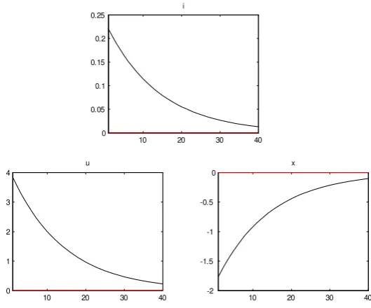
In …gure (1), (2), (3) and (4) we consider the e¤ect of a one standard de-viation, negative productivity shock on the nominal interest rate, in‡ation, the output gap and the rate of unemployment under di¤erent types of mon-etary policy. Under a policy aimed at stabilizing output, which we obtain by setting xt = 0, a negative productivity shock will imply an increase in

response of the interest rate, which will initially increase by 0.22 percentage points. The output gap will increase by 1.7 percentage points and the rate of unemployment will fall by almost 4 percentage points.

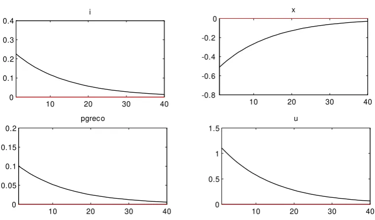
As we could expect, the optimal policy under discretion, which is de-scribed in …gure (3), stirs an intermediate course between these two extreme policies. A negative productivity shock will require an increase in the nomi-nal interest rate of 0.2% and an increase in in‡ation of almost 0.1%. Initially output will fall by 0.7% and the rate of unemployment will have an initial in-crease of about 1.5 percentage points. An optimal monetary policy, therefore, will take into account the trade-o¤ that exists between in‡ation stabilization and output stabilization: as a response to a productivity shock output will decrease less than in the extreme in‡ation targeting case and in‡ation will also increase less than in the policy aimed at fully stabilizing output and unemployment.

In …gure (4) we report the results of an exercise aimed at replicating the optimal policy through a simple Taylor rule. We found that a rule that approximates quite well the optimal monetary policy (i.e. that achieves a response of the major variables quite close to the one achieved by our economy under the optimal discretional monetary policy) is given by

it= 2:5 t+ 0:05xt (75)

for example, found a response to in‡ation equal to 2:15 and a response to unemployment equal to 0:93 . Smets and Wouters [37] for the European economy found a response to in‡ation equal to1:658and a response to output of 0:145:

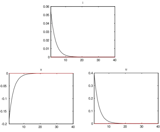
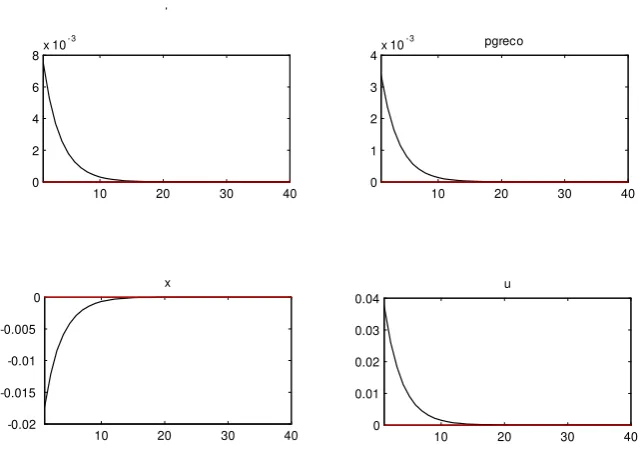
In …gure (5)-(8) we show the responses of the interest rate, output and unemployment to a one standard deviation shock to the reservation wage. The responses are quite similar to those obtained for the negative produc-tivity shock although, given the smaller persistence of the wage shock, the e¤ect lasts for fewer quarters.

6

Conclusions

in‡ation, but will also react to increases in the rate of interest supporting the e¢cient equilibrium that are not necessarily one to one. The model is also capable of accounting for the greater volatility of unemployment relative to the wage volatility that is usually found in the data.

Even though we think that the model represents a step forward in the analysis of optimal monetary policy of contemporary economies, we are aware that it gives a representation of the working of the labor market which is still quite crude. For the sake of simplicity, many other market imperfections, like search and matching costs and …ring costs are absent. Moreover, the model assumes that the whole labor market is unionized. A more realistic representation of the challenges provided to monetary policy by di¤erent in-stitutional settings in the labor market would imply considering, for example, a two sector model where only a fraction of workers belong to unions and are covered by collective agreements. We leave however these challenges to our future research.

References

[1] Anderson S., and Devereux M. (1988). Trade Unions and the Choice of Capital Stock, Scandinavian Journal of Economics 90, 27–44.

[3] Amato J. D., Laubach T. (2003). Estimation and Control of an Optimization-Based Model with Sticky Prices and Wages. Journal of Economic Dynamics and Control 27, 1181-1215.

[4] Blanchard O. and Galì J. (2006). Real Wage Rigidities and the New Keynesian Model, Journal of Money Credit and Banking, forthcoming.

[5] Blanchard O. and Galì J. (2006). A New Keynesian Model with Unem-ployment. mimeo.

[6] Calvo G. A. (1983), Staggered Prices in a Utility-Maximizing Frame-work, Journal of Monetary Economics 12(3) 383-398.

[7] Chéron A. and Langot F. (2000). The Phillips and Beveridge Curves Revisited, Economics Letters 69, 371-376.

[8] Clarida R., Galì J., Gertler M. (1999). The Science of Monetary Policy: A New Keynesian Perspective. Journal of Economic Literature, 47 (4) 1661-1707.

[9] Christo¤el K., Linzert T. (2005). The Role of Rela wage Rigidities and Labor Markets Friction for Unemployment and In‡ation Dynamics, ECB Working Paper Series n 556.

[10] Christo¤el K., Kuester K., Linzert T. (2006). Identifying the Role of Labor Markets for Monetary Policy in an Estimated DSGE Model, ECB Working Paper Series n 635.

[12] Dunlop J. T. (1944). Wage Determination under Trade Unions, London, Macmillan.

[13] Farber H. S. (1986). The Analysis of Union Behavior, in Ashenfelter O., Card D., (1986), vol. II, 1039-1089.

[14] Francis N. R., Owyang M. T., Theodorou A. T. (2005). What Explains the Varying Monetary Response to Technology Shocks in G-7 Countries?

International Journal of Central Banking, 1 (3) 33-71.

[15] Galí J. (2001), The Conduct of Monetary Policy in the Face of Tech-nological Change: Theory and Postwar U.S. Evidence, in Stabilization and Monetary Policy: the International Experience, Banco de México.

[16] Galì J., Lòpez-Salido J. D., Vallès J. (2003). Technology Shocks and Monetary Policy: assessing the Fed’s Performance,Journal of Monetary Economics, 50 723-743.

[17] Galì J., Rabanal P. (2004). Technology Shocks and Aggregate Fluctua-tions: How Well Does the RBS Model Fit Postwar U.S. Data? NBER Working Paper n 10636.

[18] Galì J., Monacelli T. (2005). Monetary Policy and Exchange Rate Volatility in a Small Open Economy, Review of Economic Studies, 72, pp. 917-946.

[20] King R., Rebelo S. T. (2000). Resusciting Real Business Cycles, Rochester Center for Economic Research, Working Paper No. 467.

[21] King R., C. Plosser, and S. Rebelo. (1988a). Production, Growth, and Business Cycles I: The Basic Neoclassical Model. Journal of Monetary Economics, 21, 195-232.

[22] Hansen G. (1985). Indivisible Labor and the Business Cycle, Journal of Monetary Economics, 16 309-328.

[23] Ireland P. N. (2004). Technology Shocks in the New-Keynesian Model,

Review of Economics and Statistics, 86(4), 923-936.

[24] Lawrence S., Ishikawa J. (2005). Trade Union Membership and Collec-tive Bargaining Coverage: Statistical Concepts, Methods and Findings, Working Paper n 59, International Labor O¢ce of Geneva.

[25] Ma¤ezzoli M. (2001.) Non-Walrasian Labor Markets and Real Business Cycles, Review of Economics Dynamics 4, 860-892.

[26] Moyen S. and Sahuc , J. G. (2005), Incorporating labour market frictions into an optimizing-based monetary policy model, Economic Modelling

22, 159-186.

[27] Oswald A. (1982). The Microeconomic Theory of the Trade Union, Eco-nomic Journal, 92, 576-595.

[29] Pissarides, C. (1998). The Impact of Employment Tax Cuts on Unem-ployment and Wages: The Role of UnemUnem-ployment Bene…ts and Tax Structure, European Economic Review 42, 155–183.

[30] Rogerson, R. (1988). Indivisible Labor Lotteries and Equilibrium, Jour-nal of monetary Economics 21, 3-16.

[31] Rogerson R., and Wright R. (1988). Involuntary Unemployment in Eco-nomics with E¢cient Risk Sharing, Journal of Monetary Economics 22, 501-515.

[32] Trigari A. (2005). Equilibrium Unemployment, Job ‡ows, and In‡ation Dynamics, ECB WP#304.

[33] Trigari A. (2006). The Role of Search Frictions and Bargaining of In‡a-tion Dynamics, mimeo.

[34] Walsh C. (2003). Labor Market Search and Monetary Shocks", in El-ements of Dynamic Macroeconomic Analysis, S. Altug, J. Chadha and C. Nolan eds.

[35] Walsh C. (2005). Labor market search, Sticky Prices, and Interest Rate Rules", Review of Economic Dynamics 8, 829-849.

[36] Woodford M. (2003). Interest and Prices: Foundations of a Theory of Monetary Policy, Princeton University Press, Princeton.

A

Technical Appendix

A.1

The Ramsey Problem

We consider a social planner which maximizes the representative household utility subject to the economy resource constraint and production function as follows:

max

Nt

U(Ct; Nt) =

1

1 C

1

t (Nt)1 (A1)

s:t: (A2)

Ct=Yt (A3)

Yt=AtNt

Substituting the constraint into the utility function the problem is:

max

N

1

1 (AtNt )

1

(Nt)1 (A4)

the …rst order condition requires

(AtNt)

Yt Nt

(Nt)1 = (AtNt )

1

(Nt) N(Nt) (A5)

simplifying

Yt N

(Nt)

(Nt)

= Yt

Nt

Multiplying both sides of equation for Nt

Yt we …nd

N(Nt)

(Nt)

Nt= (A7)

and

UN UC

Nt Yt

= N(Nt) (Nt)

Nt= (A8)

A.2

Derivation of the E¢cient Output

We consider the Ramsey solution (A17)

N(Nt)Nt = (Nt) (A9)

in order to …nd an equation for the e¢cient output we …rst log-linearizing equation (A9) around the steady state, which implies

[ N(N) + N N(N)N nt]N(1 +nt) = ( (N) + N(N)N nt) (A10)

which can be rewritten as

N(N)N+ N(N)N nt+ N N(N)N2nt= ( (N) + N(N)N nt) (A11)

Considering the steady state equation

and collecting terms in nt we obtain

1 + N(N)Nt (N) +

N N(N)N2

(N)

N(N)Nt

(N)

1!

nt= 0 (A13)

given that 1 + N(N)Nt (N) +

N N(N)N2 (N)

N(N)Nt (N)

1

6

= 0 we require,

nt= 0 (A14)

and then from the aggregate production function we obtain equation (24) in the text.

A.3

Derivation of the Flexible Price Equilibrium

Out-put in the Walrasian Model

Let us rewrite equation (25) as:

N(Nt)Nt=

(1 )M Ct (Nt) (A15)

at the steady state becomes,

N(N)N =

1

(1 ) M C (N) (A16)

Then log-linearizing,

[ N(N) + N N (N)N nt]N(1 +nt) =

M C

(1 )(1 +mct) [ (N) + N(N)N nt]

considering the steady state equation (A16) we have,

mct = 1 + N

(N)N

(N) +

N N (N)N2

(N) nt (A18)

given equation (A14) and considering the aggregate production function we obtain equation (28) in the text.

A.4

Derivation of the Phillips Curve

Following Calvo [6] we assume that each …rm may reset its price with prob-ability 1 ' each period, independently from the time elapsed since the last adjustment. This means that each period a measure1 'of …rms reset their price, while a fraction ' of them keep their price unchanged. The law of motion of the aggregate price is given by:

lnPt='lnPt 1+ (1 ') lnPt (A19)

which implies

t= (1 ') ln pt Pt 1

(A20)

wherelnPt denotes the (log) price set by a …rmiadjusting its price in period t: Under Calvo [6] price-setting structure pt+k(i) = pt with probability 'k

for k = 0;1;2; :::; hence …rms have to be forward-looking.

rule:

lnPt (i) = P

+ (1 ') 1

X

k=0

( ')kEt mcnt;t+k (A21)

where mcn

t;t+k is the log-linearized nominal marginal cost in period t+k of

a …rm which last set its price in period t: Considering the equation of real marginal cost and the one of the aggregate production function,

M Ct;t+k = (1 )

(Wt+k=Pt+k)

(Yt;t+k=Nt;t+k)

= M Ct+k

(Yt+k=Nt+k)

(Yt;t+k=Nt;t+k)

= M Ct+k

Yt+k Yt;t+k

1

= M Ct+k P_t Pt+k

1

(A22)

taking the logs

lnM Ct;t+k = lnM Ct+k

1

ln Pt Pt+k

(A23)

Considering that all …rms resetting prices in period t will choose the same price Pt+ we can rewrite equation (A21) as,

ln Pt (i) Pt 1

= P _{+ (1 ')}

1

X

k=0

( ')kEt lnM Ct;tn+k lnPt 1

= P + (1 ') 1

X

k=0

( ')kEt lnM Ct;tn+k +

+ 1

X

k=0

substituting equation (A5) which can be rewritten as

ln Pt (i) Pt 1

= P _{+ (1 ')}

1

X

k=0

( ')kEt lnM Ct;tn+k

1

ln Pt Pt+k

+ 1

X

k=0

( ')kf t+kg (A25)

then

lnPt (i) lnPt 1 = P + 'Et lnPt+1 lnPt + (1 ') lnM Ct (A26)

Combining (A26) with (A19) we obtain

t = Et t+1+ mct (A27)

as in the text.

A.5

The Welfare-Based Loss Function

A second-order Taylor expansion of the period utility around the e¢cient equilibrium yields,

Ut =Ut+UC;tCtC~t+

1

2UCC;tC

2

tC~t2+UN ;tNtN~t+

1

2UN N ;tN

2

tN~t2+

+UCN ;tCtNtC~tN~t+ k k3 (A28)

where the generic X~ = ln X=Xt denotes log-deviations from the e¢cient

equilibrium and Xt denotes the value of the variable under e¢cient

Considering the ‡exible prices economy resource constraint,

Ut = Ut+UY ;tYtY~t+

1

2UY Y ;tY

2

t Y~

2

t +UN ;tNtN~t+

1

2UN N ;tN

2

tN~

2

t +

+UY N ;tYtNtY~tN~t+ k k3 (A29)

Collecting terms yields

Ut=Ut+UY ;tYt

2

6 4

~

Yt+ U_{N ;t}Nt

U_{Y ;t}Yt

~

Nt+ 1₂ U_{Y Y ;t}

U_{Y ;t} YtY~

2

t +

+1₂UN N ;tNt2

UY ;tYt

~

Nt2+

UY N ;tNt

UY ;t

~

YtN~t

3

7

5+ k k3 (A30)

Considering that, UY N ;tNt

U_{Y ;t} =

N ;t(Nt)Nt

(Nt) = (1 ) ;we have,

Ut=Ut+UY ;tYt

2

6 6 4

~

Yt N~t ₂Y~t2+ (1 )

N(Nt)

(Nt) Nt

~

YtN~t

+1 2

"

N N(Nt)

(Nt)

N(Nt)

(Nt) 2#

N2

tN~t2

3

7 7

5+ k k 3

(A31) It can be shown that N N;t(Nt)

(Nt) =

2 1 N(Nt)

(Nt) 2

; hence

Ut=Ut+UY ;tYt

2

6 6 4

~

Yt N~t ₂Y~t2+ (1 )

N(Nt)

(Nt) Nt

~

YtN~t

+1₂

"

2 1 N(Nt)

(Nt) 2#

N2

tN~t2

3

7 7

5+ k k 3

(A32)

Ut =Ut+UY ;tYt

2

6 4

~

Yt N~t ₂Y~t2 (1 ) ~YtN~t+

+1₂ 2 1 2_N~2

t

3

7

5+ k k3 (A33)

state.

UY ;tYt=UY 1 + (1 )yt+ (1 ) N

(N)

(N) N nt + k k

2

=UY (1 + (1 )yt (1 ) nt) + k k2 (A34)

N Nt

Nt

Nt= N

(N)

(N) N + nnt+ + k k

2

(A35)

where n= N₍(N_N)₎N + N N(N)N

2 (N)

N(N)2N2 (N)2

N Nt Nt

Nt

!2

= N(N)N

2

(N)

2

+ nnt+ k k2 (A36)

where n = 2 N(N)_(NN N₎2(N)N + N (N)N

(N) 2

N(N) (N)

3

N

given that nt= 0;and that N(₍N_N)₎N = ;substituting (A35) and (A36) into

the Welfare function,

Ut =Ut+UY (1 + (1 )yt)

2

6 4

~

Yt N~t ₂Y~t2 (1 ) ~YtN~t

+1 2

2 1 2_N~2

t

3

7

5+ k k3

(A37) Given the aggregate production function and that the log-deviations of the price dispersion index dt = ~Yt N~t are of second-order, and that:

~

considering only terms up to the second-order we have:

Ut =Ut+UY

2

6 4

~

Yt N~t ₂Y~t2 (1 ) ~Yt2

+1 2

2 1 _Y~2

t

3

7

5+ k k3 (A38)

~

Ut Ut Ut= UY dt+

1 2

2 1

2 Y~2

t + k k

3

= Ut Ut= UY dt

1 2 Y~

2

t + k k

3

(A39)

As proven by Galì and Monacelli [18], the log-index of the relative-price distortion is of second-order and proportional to the variance of prices across …rms, which implies that:

dt= ln

"Z 1

0

Pt(j) Pt

dj

#

=

2vari pt(i) + k k

3

(A40)

proof Galì and Monacelli [18].

As shown in Woodford [36], this means that

1

X

t=0

t

varifpt(i)g=

1 a 1 X t=0 t 2 t (A41)

where = (1 ) (1 )= :

Welfare-Based loss-function can be written as,

Wt=Et

1

X

t=0

t_U~ t+k=

UY

2 Et 1

X

t=0 a

2

t+k+

1

xt+k + k k3

=Et

1

X

t=0

t_~ Ut+k=

UY

2 Et 1

X

t=0 a

2

t+k+

1

xt+k + k k3 (A42)

A.6

Stability and Determinacy in the Reduced Form

Dynamic System

Our model can be expressed in the following reduced form:

xt = Etxt+1 [rt Et t+1 r^nt] (A43)

t = Et t+1+ a

1

xt+

a

(1 _a)r^

n

t + awrt (A44)

the model is completed adding the optimal instrument rule interest rate which, under discretion is given by:

^

rt = Et t+1+ rr^tn (A45)

where = 1 + 1 w w

1 _and

r = 1 + (₍₁a w)

a) a:

dynamic system:

xt = Etxt+1+ (1 )Et t+1+ (1 r)rnt (A46)

t = a

1

Etxt+1+ a

1

(1 ) + Et t+1+

+ 1 + a

(1 a)

r rnt + awrt (A47)

which can be rewritten as

$t=A1Et$t+1+A2ut (A48)

where$t =Et[xt; t]T andAT2 = 2

6 4

1 r 0

1 + _{(1 a)} r a

3

7

5; ut= [rnt; wtr] T

while the transition matrix is given by:

A1 = 2

6 4

1 1

a1 a1 (1 ) +

3

7

5 (A49)

Given that $t is a 2-vector of non-predetermined endogenous variable,

rational expectation equilibrium is determinate if and only if the matrix A1 has both eigen values outside the unit circle, which occurs if and only if13_:

detA1 <1; (A50)

j trA1j<1 + detA1: (A51)

Notice that, in our case:

detA1 = a

1

(1 ) + a

1

(1 ) = <1 (A52)

j trA1j= 1 + a

1

(1 ) + <1 + given that >1 (A53)

which implies that the rational expectations equilibrium of our model under an optimal discretionary policy is determinate.

The optimal instrument rule commitment is given by:

^

rc

t = cEt t+1+ crr^nt (A54)

where c _{= 1 +} 1

1 1 and

c r= 1:

Under commitment matrix A1 becomes:

A1 = 2

6 4

1 1 c

a1 a1 (1 c) +

3

7

5 (A55)

Notice that

detA1 = a

1

(1 c) + a

1

j trA1j= 1 + a

1

(1 c_{) + <1 + given that} c _{>1 (A57)}

Tables and Figures

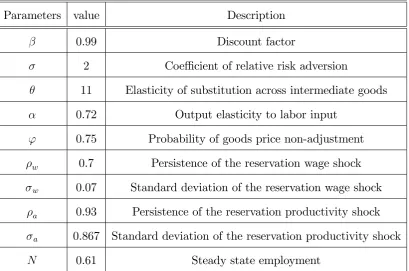
Table 1.

Parameters value Description

0.99 Discount factor

2 Coe¢cient of relative risk adversion

11 Elasticity of substitution across intermediate goods 0.72 Output elasticity to labor input

' 0.75 Probability of goods price non-adjustment

5 10 15 20 25 30 35 40 0

0.1 0.2 0.3 0.4

i

5 10 15 20 25 30 35 40

0 0.05 0.1 0.15 0.2

pgreco

Figure 1: IRFs to a negative productivity shocks under constant output

10 20 30 40

0 1 2 3 4

u

10 20 30 40

-2 -1.5 -1 -0.5 0

x

10 20 30 40

0 0.05 0.1 0.15 0.2 0.25

i

10 20 30 40 0

0.05 0.1

pgreco

10 20 30 40

0 0.05 0.1

re

10 20 30 40

0 0.1 0.2 0.3 0.4 i

10 20 30 40

0 0.5 1 1.5 2 u

10 20 30 40

-0.8 -0.6 -0.4 -0.2 0 x

Figure 3: IRFs to a negative technology shock under the optimal interest rate rule

10 20 30 40

0 0.05 0.1 0.15 0.2 pgrec o

10 20 30 40

0 0.5 1 1.5

u

10 20 30 40

0 0.1 0.2 0.3 0.4 i

10 20 30 40

-0.8 -0.6 -0.4 -0.2 0 x

5 10 15 20 25 30 35 40 0

1 2 3 4x 10

-3 _pgreco

5 10 15 20 25 30 35 40

0 1 2 3x 10

-3 _i

Figure 5: IRFs to a positive reservation wage shock under a constant output rule

10 20 30 40

-0.2 -0.15 -0.1 -0.05 0

x

10 20 30 40

0 0.1 0.2 0.3 0.4

u

10 20 30 40

0 0.01 0.02 0.03 0.04 0.05 0.06

i

10 20 30 40 0

1 2 3 4x 10

-3 _pgreco

10 20 30 40

0 0.02 0.04 0.06

u

10 20 30 40

-0.03 -0.02 -0.01 0

x

10 20 30 40

0 0.005

0.01 0.015

i

Figure 7: IRFs to a positive reservation wage shock under the optimal interst rate rule

10 20 30 40

0 2 4 6 8x 10

-3

i

10 20 30 40

0 1 2 3 4x 10

-3 _pgreco

10 20 30 40

0 0.01 0.02 0.03 0.04 u

10 20 30 40

-0.02 -0.015 -0.01 -0.005 0 x