On Optimal Ordering of Service Parameters of a Coxian Queueing Model with Three Phases

(1)

http://dx.doi.org/10.4236/ojop.2015.43008

On Optimal Ordering of Service Parameters

of a Coxian Queueing Model with Three

Phases

Vedat Sağlam1, Murat Sağır1, Erdinç Yücesoy1, Müjgan Zobu2

1_{Department of Statistics, Ondokuz Mayıs University, Samsun, Turkey} 2_{Department of Statistics, Amasya University, Amasya, Turkey}

Email: [email protected], [email protected], [email protected],

[email protected]

Received 8 June 2015; accepted 23 August 2015; published 26 August 2015

This work is licensed under the Creative Commons Attribution International License (CC BY). http://creativecommons.org/licenses/by/4.0/

Abstract

We analyze a Coxian stochastic queueing model with three phases. The Kolmogorov equations of this model are constructed, and limit probabilities and the stationary probabilities of customer numbers in the system are found. The performance measures of this model are obtained and in addition the optimal order of service parameters is given with a theorem by obtaining the loss probabilities of customers in the system. That is, putting the greatest service parameter at first phase and the second greatest service parameter at second phase and the smallest service para-meter at third phase makes the loss probability and means waiting time minimum. We also give

the loss probability in terms of mean waiting time in the system. αj is the transition probability

from j-th phase to

(

j+1

)

-th phase

(

j=1, 2

)

. In this manner while α1=0 and α2≥0 this

sys-tem turns into M M 1 0| | | queueing model and while α₁≥0,α₂ =0 the system turns into Cox(2)

queueing model. In addition, loss probabilities are graphically given in a 3D graph for corres-ponding system parameters and phase transient probabilities. Finally it is shown with a numeric example that this theorem holds.

Keywords

Stochastic Coxian Queueing Model, Loss Probability, Limiting Distribution, Optimization, Kolmogorov Equations

1. Introduction

(2)

need to construct phase-type distributions for complex representations of queueing models. The recent works being done in this field are: D. R. Cox shows how any distribution having a rational Laplace transform can be represented by a sequence of exponential phases [1]. S. Asmussen, O. Nerman and M. Olsson gave a paper on fitting phase-type distributions with the EM Algorithm [2]. Q. -M. He and H. Zhang presented an algorithm for computing minimal ordered Coxian representations of phase-type distributions whose Laplace-Stieltjes trans-form had only real poles [3]. The optimal ordering of the tandem server with two stages is given by [4]. R. Ma-rie studied on calculating equilibrium probabilities for Coxian queueing systems in [5]. X. A. Papaconstantinou analyzed the stationary Ek/C2/s queueing system in [6]. P. M. Snyder and W. J. Stewart considered two

ap-proaches to the numerical solution of single node queueing models with phase-type [7]. In [8], an exact analysis of a fork/join station in a closed queueing network with inputs from servers with two-phase Coxian service dis-tributions is represented. Q. -M. He and H. Zhang studied the approximation of matrix-exponential disdis-tributions by Coxian distributions in [9]. M. Fackrell gave a survey of where the phase-type distributions were used in the healthcare industry and purposed some ideas on how they were further utilized [10]. A. B. Zadeh studied a batch arrival queue system with Coxian-2 server vacations and admissibility restricted in [11]. V. Sağlam et al. give a paper on optimization of a Coxian queueing model with two phases in [12].

There is not enough work on the studies of optimizing the orders of service parameters for Coxian queueing model so far. Considering this fact in this paper we analyze a Coxian stochastic queueing model with three phases, and the Kolmogorov equations of this model are constructed, limit probabilities and the stationary prob-abilities of customer numbers in the system are found. The performance measures of this model are obtained and in addition the optimal order of service parameters is given by a theorem by obtaining the loss probabilities of customers in the system. We also give the loss probability in terms of mean waiting time in the system. Finally it is shown with a numeric example that this theorem holds.

2. Stochastic Model

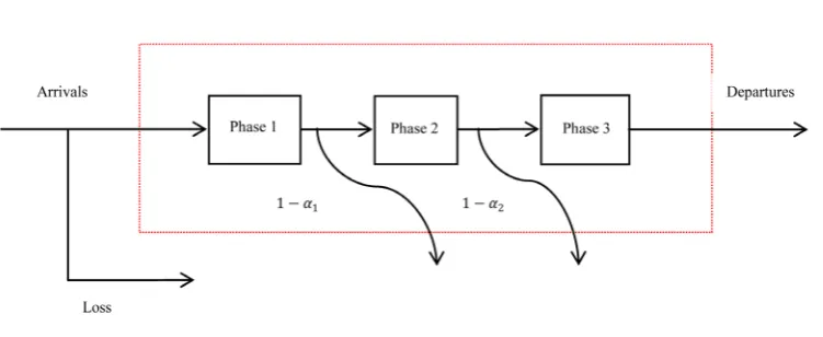
We have obtained stochastic equation systems of a Coxian queueing model with three servers in which the stream is Poisson with λ parameter. The service time of any customer at server i

(

i=1, 2, 3

)

is exponential with

parameter µi. Two or more customers can not have service in the system at the same time. Let ξt be the state

of server 1, ηt be the state of server 2 and ζt be the state of server 3 at any t time. αj is the transition

prob-ability from j th- phase to

(

j+1 -

)

th phase

(

j=1, 2

)

and 1 − αi be the loss probability of the system. This

stochastic queueing model is illustrated inFigure 1. Limit probabilities, differential and difference equations of this system given later.

Limit Probabilities

Here

{

(

ξ η ζt, t, t

)

,t≥0

}

is a three-dimensional Markov chain with continuous parameter and state space is Ω =

{

(

0, 0, 0 , 1, 0, 0 , 0,1, 0 , 0, 0,1

) (

)

}

( )

{

} (

)

1, 2,3 1, 2, 3 , 1, 2, 3

n n n t t t

[image:2.595.127.503.551.705.2]

p t =Prob ξ =n η =n ζ =n ∀ n n n ∈ Ω (1)

(3)

Kolmogorov differential equation for these probabilities is obtained. The probabilities of the process

(

)

{

ξ η ζt, t, t ,t≥0

}

will be found for

(

t t, +h

)

, namely

(

)

(

( )

)

( ) (

)

(

( )

)

( )

(

)

(

( )

)

( )

(

( )

)

( ) ( )

(

)

(

( )

)

( )

(

( )

)

( ) ( )

(

)

(

( )

)

( )

(

( )

)

( ) ( )

(

)

(

( )

)

( )

(

( )

)

( ) ( )

000 000 1 1 100

2 2 010 3 001

100 1 100 000

010 2 010 1 1 100

001 3 001 2 2 010

1 1

1 0 0

1 1 1

p t h h o h p t h o h p t

h h p t h h p t o h

p t h h o h p t h o h p t o h

λ α

α

µ λ

µ α µ

µ α µ µ µ µ + = − + + − + + − + + + + + = − + + + + + = − + + + + + = − + + + + (2)

We write Equation (2) as follows as h→0

( )

( ) (

)

( ) (

)

( )

000 000 1 1 100 2 2 010 3 001

100 1 100 000

010 2 010 1 1 100

001 3 001 2 2 010

1 1

p t p t p t p t p t

p t p t p t

λ α α

λ α

µ µ µ

µ µ µ µ α µ ′ = − + − + − + ′ = − + ′ = − + ′ = − + (3)

Furthermore, it is supposed that limiting distribution of

( )

1,2,3

n n n

p t are exist as follow:

( )

1,2,3 1,2,3 1,2,3

lim _{n n n} _{n n n} , lim _{n n n} 0 t→∞p t p t→∞p t

′

= = . (4)

Steady-state equations for

{

(

ξ η ζt, t, t

)

,t≥0

}

are obtained as following:

(

)

(

)

000 1 1 100 2 2 010 3 001

1 100 000 2 010 1 1 100 3 001 2 2 010

0 1 1

0 0 0

p p p p

p p

p P

λ α µ α µ µ

µ λ

µ α µ µ α µ

= − + − + − +

= − +

(5)

( ) 1 2 3 1 2 3

, , , ,

1

n n n n n n

p

∈Ω

=

∑

(6)

We define ρi =λ µi,

(

i=1, 2, 3 .

)

If we solve Equation (5) under condition (6), we obtain the following

three dimension probability function:

(

)

(

)

(

) (

)

(

) (

)

1 2 3

1 2 3 1 1 2 1 2 3

1

1 2 3 1 1 2 1 2 3

1 2

1 2 3 1 1 2 1 2 3

1 2 3

1 2 3 1 1 2 1 2 3

1

, , , (0, 0, 0) 1

, , , (1, 0, 0) 1

, , , 0,1, 0

1

, , , 0, 0,1

1

0, otherwise

n n n

p n n n

n n n

ρ α ρ α α ρ ρ

ρ α ρ α α ρ α ρ

ρ α ρ α α ρ α α ρ ρ α ρ α α ρ

 ₌  + + +   =  + + +   =_ = + + +   =  + + +     (7)

3. Obtaining the Measures of Performance

Let 𝑁𝑁 be the random variable that describes the number of customers in the system. The mean number of cos-tumers:

[ ]

( )

(

)

1 2 3

1 1 2 1 2 3

1 2 3

, , 1 1 1 2 1 2 3

n n n n n n

E N n n n p ρ α ρ α α ρ

ρ α ρ α α ρ

∈Ω

+ +

= + + =

+ + +

(4)

[ ]

(

)

2 2

2

1 1 2 1 2 3 1 1 2 1 2 3

1 1 2 1 2 3 2 1 1 2 1 2 3

1 1

1

Var N E N E N

ρ α ρ α α ρ ρ α ρ α α ρ

 

= _ _−

 

+ + + +

= _{− } _

+ + + _ + + + _

+ +

=

+ + +

. (9)

3.1. The Coxian Queue Using Laplace Transform

Let W be the random variable that describes waiting time of customers in the system. Laplace transform of W

( ) (

1

)

1 1 1

(

2

)

2 1 1 2 2 3

1 1 2 1 2 3

1 1

W s

s s s s s s

α µ α µ α µ α µ α µ µ

µ µ µ µ µ µ

− −

= + +

+ + + + + +

 . (10)

Mean waiting time in system of a customer for Cox(3) is found by formula (10)

[ ]

( )

1 1 2

1 2 3

0

d 1

d

W

s

s E W

s

α α α µ µ µ

=

= −  = + + (11)

3.2. The optimization of Measures of Performance

Loss probability

Let Ploss be the loss probability of customer in the system. In this regards, since there is no queue in the

sys-tem, loss probability is calculated as following:

loss 100 010 001

P = p + p +p . (12)

3.3. Optimal Order of Servers

We can put three different service parameters to three stages in 3! different position. In this case there are 6 dif-ferent loss probabilities.

The following theorem is given on minimization of loss probability.

Theorem 1. Putting the greatest service parameter at first phase and the second greatest service parameter at second phase and the smallest service parameter at third phase makes the loss probability minimum. That is,

( )1 ( )

, 2, , 6

i loss loss

P ≤P i=  (13)

Proof. Let’s suppose µ1≥µ2 ≥µ3. In this case we have,

2 3

1 1

0

µ µ

 

− ≤

 

 

(

)

1 2

2 3

1 1

1 0

α α

µ µ

 

−  − ≤

 

1 1 2 1 1 2

2 3 3 2

α α α α α α

µ + µ ≤µ + µ

1 2 1 2 3 1 3 1 2 2 α ρ +α α ρ ≤α ρ α α ρ+

1 1 2 1 2 3 1 1 3 1 2 2 ρ α ρ+ +α α ρ ≤ρ α ρ α α ρ+ +

1 1 2 1 2 3 1 1 3 1 2 2

1 1

+ ≥ +

+ + + +

1 1 2 1 2 3 1 1 3 1 2 2

1 ρ α ρ α α ρ 1 ρ α ρ α α ρ

+ + + + + +

≥

(5)

( )1 ( )2 loss loss

P ≤P .

Similarly,

(

1

)

1 2

1 1

1 α 0

µ µ

 

− _ − _≤

 

1 1

1 2 2 1

1 α 1 α

µ +µ ≤µ +µ

1 1 2 1 2 3 2 1 1 1 2 3 ρ α ρ+ +α α ρ ≤ρ +α ρ α α ρ+

1 1 2 1 2 3 2 1 1 1 2 3

1 1

+ ≥ +

+ + + +

1 1 2 1 2 3 2 1 1 1 2 3

+ + + + + +

≥

+ + + +

( )1 ( )3 loss loss

P ≤P .

Since,

(

)

(

)

1 2 1

1 3 1 2

1 1 1 1

1 1 0,

α α α

µ µ µ µ

   

− _ − _+ − _ − _≤

 

we obtain

1 1 2 1 1 2

1 2 3 2 3 1

1 α α α 1 α α α

µ +µ + µ ≤ µ +µ + µ

1 1 2 1 2 3 2 1 3 1 2 1 ρ α ρ+ +α α ρ ≤ρ +α ρ α α ρ+

1 1 2 1 2 3 2 1 3 1 2 1

+ + + + + +

≥

+ + + +

( )1 ( )4 loss loss

P ≤P .

(

1

)

1

(

2

)

1 3 2 3

1 1 1 1

1 α α 1 α 0

µ µ µ µ

   

− _ − _+ − _ − _≤

   

1 1 2 1 1 2

1 2 3 3 1 2

1 α α α 1 α α α

µ +µ + µ ≤µ +µ + µ

1 1 2 1 2 3 3 1 1 1 2 2 ρ α ρ+ +α α ρ ≤ρ α ρ α α ρ+ +

1 1 2 1 2 3 3 1 1 1 2 2

+ + + + + +

≥

+ + + +

( )1 ( )5 loss loss

P ≤P .

Finally,

(

1 2

)

1 3

1 1

1 α α 0

µ µ

 

− _ − _≤

 

1 2 1 2

1 3 3 1

1 α α 1 α α

(6)

1 1 2 1 2 3 3 1 2 1 2 1 ρ α ρ+ +α α ρ ≤ρ α ρ+ +α α ρ

1 1 2 1 2 3 3 1 2 1 2 1

+ + + + + +

≥

+ + + +

( )1 ( )6 loss loss

P ≤P

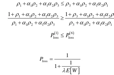
Corollary. Since,

[ ]

loss

1 1 1

P

E W

λ

= +

(14)

the minimum value which makes Ploss minimum also makes E W

[ ]

mininmum.

4. Numerical Example

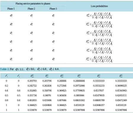
In this section the loss probabilities are calculated for some values of system probabilities and α α1, 2

probabil-ities. The calculated loss probabilities are given in Table 1. For the values λ=2.2, µ1=8.6; µ2=6.8, 3 4.4

µ = and for various values of α₁andα₂ it is seen in Table 1 that P_loss( )1 has its minimum value, this shows that Theorem1 holds.

Under condition given in Theorem1, for the values λ=2.2, µ1=8.6; µ2=6.8, µ3=4.4 and for all

[image:6.595.204.403.86.217.2] [image:6.595.99.533.488.699.2]

values of α1andα2 in domain set, the loss probabilities are calculated inTable 2 and graphically given in 3D Figure 2 in two different view angle. P_loss( )1 is indicated by green surface in this figure. As it is seen in this graph, Ploss( )1 is minimum for all values of α1andα2. For a customer to have service at each stage it must be

1 2 1

α =α = or it must be α1=0 for the customer to leave the system after first stage.

5. Conclusion

By constructing this stochastic queueing model, transient probabilities are obtained. Depending on these proba-bilities, mean number of customer in the system, the mean waiting time in this system by Laplace transform and the loss probability of any customer are given. It is shown by Theorem 1 that putting the greatest service parameter at first phase and the second greatest service parameter at second phase and the smallest service parameter at third phase makes the loss probability minimum. For the values λ=2.2, µ1=8.6; µ2=6.8, µ3=4.4 and

(7)

Table 1. Placing the service parameters to phases and corresponding loss probabilities.

Placing service parameters to phases

Loss probabilities

Phase 1 Phase 2 Phase 3

1

µ µ2 µ3

( )1 1 1 2 1 2 3

loss

1 1 2 1 2 3 1

P ρ α ρ α α ρ ρ α ρ α α ρ

+ +

=

+ + +

1

µ µ3 µ2

( )2 1 1 3 1 2 2

loss

1 1 3 1 2 2 1

+ +

=

+ + +

2

µ µ1 µ3

( )3 2 1 1 1 2 3

loss

2 1 1 1 2 3 1

+ +

=

+ + +

2

µ µ3 µ1

( )4 2 1 3 1 2 1

loss

2 1 3 1 2 1 1

+ +

=

+ + +

3

µ µ1 µ2

( )5 3 1 1 1 2 2

loss

3 1 1 1 2 2 1

+ +

=

+ + +

3

µ µ2 µ1

( )6 3 1 2 1 2 1

loss

3 1 2 1 2 1 1

+ +

=

[image:7.595.87.538.98.481.2]

+ + +

Table 2. For λ =2.2, µ =1 8.6; µ2=6.8, µ3=4.4.

1

α α2

( )1 loss

P ( )2

loss

P ( )3

loss

P ( )4

loss

P ( )5

loss

P ( )6

loss P

0 0 0.203703 0.203704 0.244444 0.24444444 0.33333333 0.33333333

0.2 0 0.242722 0.262436 0.272564 0.29752066 0.35532233 0.36090225

0.4 0.8 0.352845 0.358704 0.369425 0.37709835 0.4137837 0.41563943

0.5 0.5 0.351734 0.36976 0.365658 0.3893066 0.41479035 0.42053111

0.8 0.4 0.402855 0.431606 0.407646 0.44610302 0.44695789 0.45672369

1 0 0.366825 0.430464 0.366825 0.4516129 0.43046357 0.4516129

1 1 0.519078 0.519079 0.519079 0.51907894 0.51907894 0.51907894

for various values of α1andα2 it is seen in Table 1 that

( )1 loss

P has its minimum value, this shows that Theo-rem1 holds. In the case α1=α2=1, the loss probabilities are all equal to each other. This is seen in both Table 1 and Graph 1. While α1=0 and α2≥0 this system turns into M M| | 1 | 0 | queueing model and while

1 0, 2 0

α ≥ α = the system turns into Cox(2) queueing model. For further studies, higher moments of meanwait-ing time in the system can be obtained and by usmeanwait-ing these moments some various statistical measures can be calculated such as variance, skewness, kurtosis and coefficient of variation. Also this model can be expanded to

k-phases.

References

[1] Cox, D.R. (1955) A Use of Complex Probabilities in the Theory of Stochastic Processes. Mathematical Proceedings of the Cambridge Philosophical Society, 51, 313-319.http://dx.doi.org/10.1017/S0305004100030231

[2] Asmussen, S., Nerman, O. and Olsson, M. (1996) Fitting Phase-Type Distributions via the EM Algorithm. Scandina-vian Journal of Statistics, 23, 419-441.

[3] He, Q.M. and Zhang, H. (2007) An Algorithm for Computing Minimal Coxian Representations. INFORMS Journal on Computing, 20, 179-190.

(8)

[5] Marie, R. (1980) Calculating Equilibrim Probabilities for λ( )n /Ck/1 /N Queues. ACM Sigmetrics Performance

Evaluation Review, 9, 117-125.

[6] Bertsimas, D.J. and Papaconstantinou, X.A. (1988) Analysis of the Stationary Ek/C2/s Queueing System. Euro-pean Journal of Operational Research, 37, 272-287.http://dx.doi.org/10.1016/0377-2217(88)90336-0

[7] Snyder, P.M. and Stewart, W.J. (1985) Explicit and Iterative Numerical Approaches to Solving Queueing Models. Op-erations Research, 33, 183-202.http://dx.doi.org/10.1287/opre.33.1.183

[8] Krishnamurthy, A., Suri, R. and Vernon, M. (2004) Analysis of a Fork/Join Synchronization Station with Inputs from Coxian Servers in a Closed Queueing Network. Annals of Operations Research, 125, 69-94.

http://dx.doi.org/10.1023/B:ANOR.0000011186.14865.19

[9] He, Q.M. and Zhang, H. (2007) Coxian Approximations of Matrix-Exponential Distributions. Calcolo, 44, 235-264. http://dx.doi.org/10.1007/s10092-007-0139-7

[10] Fackrell, M. (2009) Modelling Healthcare Systems with Phase-Type Distributions. Health Care Management Science, 12, 11-26.http://dx.doi.org/10.1007/s10729-008-9070-y

[11] Zadeh, A.B. (2012) A Batch Arrival Queue System with Coxian-2 Server Vacations and Admissibility Restricted.

American Journal of Industrial and Business Management, 2, Article ID: 18843.