Multiple Node Placement Strategy for Efficient Routing in Wireless Sensor Networks

http://dx.doi.org/10.4236/wsn.2015.78009

Multiple Node Placement Strategy for

Efficient Routing in Wireless

Sensor Networks

Kirankumar Y. Bendigeri

_{, Jayashree D. Mallapur}

1_{Department of Electronics, Jain University Bangalore, Karnataka, India}

2_{Department of Electronics & Communication Engineering, Basaveshwar Engineering College, Bagalkot,} Karnataka, India

Email: kiranbendigeri@gmail.com, bdmallapur@yahoo.co.in

Received 21 May 2015; accepted 24 August 2015; published 27 August 2015

Copyright © 2015 by authors and Scientific Research Publishing Inc.

This work is licensed under the Creative Commons Attribution International License (CC BY). http://creativecommons.org/licenses/by/4.0/

Abstract

The advances in recent technology have lead to the development of wireless sensor nodes forming a wireless network, which over the years is used from military application to industry, household, medical etc. The deployment pattern of sensor nodes in Wireless Sensor Network (WSN) is always random for most of the applications. Such technique will lead to ineffective utilization of the net-work; for example fewer nodes are located at far distance and dense nodes are located at some reason and part of the region may be without the surveillance of any node, where the networks do consume additional energy or even may not transfer the data. The proposed work is intended to develop the optimized network by effective placement of nodes in circular and grid pattern, which we call as uniformity of nodes to be compared with random placement of nodes. Each of the nodes is in optimized positions at uniform distance with neighbors, followed by running a energy effi-cient routing algorithm that saves an additional energy further to provide connectivity manage-ment by connecting all the nodes. Simulation results are compared with the random placemanage-ment of nodes, the residual energy of a network, lifetime of a network, energy consumption of a network shows a definite improvement for uniform network as that of with the random network.

Keywords

Energy Consumption, Network Lifetime, Node Deployment, Connectivity Management

1. Introduction

importance in the current trends because of various advantages as compared with other networks. Sensors are capable of sensing the data, processing and transmitting with wireless communication. The data can be frag-mented into sub units so as to be transmitted from multiple sensors that consider the load balancing. The recent advances in MEMS [1], nano technology, various processors, and wireless communication have lead to the ad-vancement of WSN which are self configuring, flexible and scalable. Its intervention is most useful when human reach ability is too difficult. The deployment of sensors can be static or a random but yet a fast response. For example in a military application, it is difficult to reach the specified areas so as to practically place the sensors, in that case sensors are randomly thrown from an area above the ground; another case would be the scenario of an agricultural application which requires structured monitoring, where sensors are uniformly distributed to re-ceive the data at regular intervals. WSN can be treated as distribution of nodes for a particular task. Sensor nodes are battery powered and are expected to operate without attendance for a relatively long period of time. Power is consumed for sensing, communicating and data processing. Sensors are also able to renew their energy from solar sources, temperature differences, or vibration. An analog signal produced by the sensors is converted to digital by an ADC and sent to controllers for further processing. Usually sensor node is independent, small in size and adaptive to the environment, and should consume extremely low energy. Sensors are responsible for collecting the data [1], where in ADC sends the type of data sensed by sensor to the processor and requests, what to be done by sensor. WSN can establish the network on its own, which usually consists of low cost, low power, low energy features, where the data transfer through these is done efficiently by various techniques in order to increase the network lifetime. It is always referred by most of the researchers that WSN uses maximum communication energy for communication, which intently can be considered as, sensor node can be made to use minimum energy to reach the neighbors thus trying to save the energy consumed. This technique can be very effective utilization to save the energy during sleep, idle and receive mode, and there is always a chance of death of node and hence the network should sustain itself to the current load or sometimes entry of new node into the network where WSN should withstand the changes for the newer nodes providing scalability. While guarantee-ing good performance overall, the sensor nodes are battery powered optimized positions along with the routguarantee-ing protocols to be designed for sensors so as to consume minimal energy extending the network lifetime. As the placement of node is an important phenomenon, if done efficiently followed by energy routing protocol, such network can greatly enhance the network lifetime.

The prime objective of sensor node is to sense the data and send it to base station or the cluster heads, and these can be considered as a communication range of several orders by which the data moment is done; it is al-ways preferred that data can alal-ways be transferred by hop to hop that is source and destination involves certain neighbors for the data moment. Energy is an important issue for WSN to prolong the network lifetime; hence effective utilization of the battery should be done to do so. It is considered that placement strategy is going to be an important strategy for WSN since effective utilization of the network can be done by having controlled place- ment of nodes, where the node positions are known which when compared with the random placement technique, where sometimes nodes are placed in a such a way that it is nearly far from the region to reach the neighboring nodes, thus leading to un effective utilization of such nodes in the network. The proposed work is intended to concentrate on the different placement of nodes like random, circular and grid based scenario of a network that is mainly worked out to save the energy consumed by the network on par with sensor nodes and to increase the network lifetime.

2. Related Work

effective communication in limited periods. The energy constraint of WSNs makes energy saving the most im-portant objective of various routing algorithms. In this paper the author presents survey of routing protocols and algorithms used in WSN’s with energy efficiency as the main goal. In WSN, [4] the sensor nodes have a limited transmission range, and their processing and storage capabilities as well as their energy resources are also li-mited. Routing protocols for wireless sensor networks are responsible for maintaining the routes in the network and have to ensure reliable multi-hop communication under these conditions. In this paper, author presents a survey of routing protocols for WSN and compares their strengths and limitations. In this paper [5] author presents a multi-objective optimization methodology for node placement in wireless sensor network design. Emerging computational intelligence leads to optimization of NP-hard problem in a simple way, differential evolution approach is used as a tool for optimization of most important parameters in node placement process of wireless sensor network. Optimal operational modes of the nodes in order to minimize the energy consumption and meet application-specific requirements have been investigated and also other optimizations have been done on clustering and communication range of sensors.

In this paper, [6] author presents how to place SNs by use of a minimal number to maximize the coverage area when the communication radius of the SN is not less than the sensing radius, which results in the applica-tion of regular topology to WSNs deployment. With nodes placed at an equal distance and equipped with an equal power supply, the energy imbalance problem and the mathematical formulation for maximizing network lifetime in grid-based WSNs are given. Author also generalizes the maximizing network lifetime problem to the randomly-deployed WSNs which shows the significance of mathematical formulation for this crucial problem. In this paper, [7] author formulates a constrained multivariable nonlinear programming problem to determine both the locations of the sensor nodes and data transmission pattern. The two objectives studied in the paper are to maximize the network lifetime and to minimize the application-specific total cost, given a fixed number of sensor nodes in a region with certain coverage requirement. Through numerical results, author shows that the optimal node placement strategies provide significant benefit over a commonly used uniform placement scheme. The author presents [8] a novel algorithm for autonomous deployment of active sensor networks. The algorithm aims to enhance the sensing coverage based on an initial placement of sensor nodes. The sensing regions are modeled as circular discs of variable sensing range limits. Based on the fact that a unique circle packing exists satisfying any given set of combinatorics and boundary conditions of a sensor network, minimum sensing range required for every interior nodes to fulfill such packing conditions can be done. Based on a number of numerical simulations, we have verified that the proposed algorithm always yields sensor deployments of wide coverage and minimize the sensing ranges required for every interior sensing node to satisfy the packing and boundary conditions. In this paper, [9] the author proposes to deploy sensors either with variable battery capacities or with non-uniform densities in order to counterbalance the non-uniform energy drainage, thus achieving a longer net-work lifetime. Monitoring region is concentric ring areas and deployed nodes in these areas such that the highest battery resources are allocated to the ring where the highest energy drainage takes place. Results show 6 to 7 times longer lifetime values are attained without any increase in costs with this approach.

de-termines the optimum node coordination of sensor nodes topology. The topology is in linear array, aimed for beam-forming in WSN’s. The array is constructed in random sensor node deployment. The selected nodes should align similar to a uniform linear array (ULA) to minimize the position errors which will improve the beam- forming performance (gain, transmission range and characteristics). Instead of utilizing random beam-forming which needs a large number of sensor nodes to interact with each other and form a narrow radiation beam, the proposed approach is emphasized to only a number of sensor nodes which can construct a linear array. Beam- forming technologies can increase the system performance, increase the transmission range and control the di-rectionality of the reception or transmission of a signal. The proposed work utilizes beam-forming technique by using ULA to establish a communication link in a WSN. In this paper [14], author proposes a systematic framework for choosing the minimum sensor nodes from those which are originally distributed randomly in a sensor network. Integer linear programming model is used to describe the optimal placement. A greedy algo-rithm is proposed under quite general conditions. Simulation results and theoretical analysis with different grid density shows that proposed framework is computationally feasible and the resultant sensor node placement performs near-optimum.

In this paper [15], environmental monitoring applications are considered where data may be continuously re-ported with the possibility of urgent alarming if necessary. Hierarchical architecture of the network is assumed in order to overcome the problem of energy constrained sensors. Two algorithms are proposed with the purpose of network lifetime elongation and the maximization of the use of the available energy. The first algorithm is a modification for LEACH-C to enhance its performance. It results in a 25% longer lifetime. The second algo-rithm is an energy efficient method to ensure full coverage of the network as long as sensors are still working. This achieves 32% longer lifetime than LEACH-C. This paper [16] presents a method of optimizing sensor node co-ordination in order to reassign the nodes in linear arrangement to form a linear antenna array. This linear sensor node array (LSNA) is constructed within random sensor node placement. The LSNA should be optimized as closely comparable as a conventional uniform linear array (ULA) to minimize the beam-forming performance errors. Beam-forming has been introduced in wireless sensor network in order to increase the transmission range of individual sensor nodes. Performance of LSNA demonstrates an excellent agreement over ULA. The posi-tioning of nodes [17] in a sensor network has an effect in its performance. In this paper, two predefined confi-gurations are compared to the random distribution to gauge the magnitude of the effect on energy consumption of each type of sensor allocation. The experiments assume a flat, obstacle free, rectangular field, with Directed Diffusion used as routing protocol, and random different positions for the querying entity (sink) and the event location in the field. The results confirm that in an environment such as this, it is worth investing in the uniform positioning of sensors as they offer a significant performance gain.

energy consumption compared to existing energy-efficient protocols developed for this network.

3. Implementation

The implementation for node deployment and best routing analysis is done in this section. We have considered three different node deployments for our experimentation and results. The Figure 1 shows the uneven distribu-tion of nodes. Node placement is a technique to place the nodes effectively in a simuladistribu-tion area so as to consume the minimum energy from each node that is intended for transmission of packets or a data. The present research is on deployment of wireless sensor nodes that are mainly concentrated in the static and the dynamic manner. In static deployment, nodes are fixed, whereas in dynamic deployment of nodes, the nodes are mobile. For the dis-cussion we have classified the static deployment into, non deterministic (random) and deterministic deployment. Randomized sensor placement often becomes the only option for WSN. Consider an example, in applications of WSN’s in reconnaissance missions during combat, disaster recovery and forest fire detection. It is widely ex-pected that sensors will be dropped by helicopter, grenade launchers or clustered bombs. Such means of dep-loyment lead to random spreading of sensors. Although the node density can be controlled to some extent.

As with most of the research that have been carried out, communication network of WSN is always consi-dered deploying the nodes with randomness. The randomness is a function to deploy the nodes randomly leading uneven or unequal distribution of nodes. When such network with the nodes that are deployed randomly is con-sidered for the simulation, there are three issues that mainly arise, some nodes are densely deployed at particular region while the other region is distributed with only fewer nodes located at farer distances and leaving region will not at all be with the single coverage of node. The drawbacks of such random node deployment is that nodes with dense location, where routing is to take place, additional hops between source and destination in a region of dense location of nodes take part in routing leading to additional utilization of energy from each node, where as in the case of nodes at far location, additional energy again is to be spent in transmitting the data to neighbors located at far distance as well to the destination which is located at quite far distances. On a similar way it is difficult to manage the routing in a region where no nodes are located leading in all the three case, an uneven distribution of energy source and node deployment. Figure 1 show the probability of random deploy-ment of sensor node network, the node pattern is set in a simulation environdeploy-ment. As shown in Figure 1, the random function distributes the nodes close to each other for example node ID, 25, 30, 85, 79, 55, 48 are all closely located and node 77, 86 are located at a such far distance that they may not be in a communication range leading to loss of data transfer or finding more additional neighbors or energy to complete the routing. Such drawback can be overcome by placing the nodes uniformly in a simulation area which we call it as deterministic node deployment.

In Deterministic Sensor Placement Schemes (DSPS), the nodes are placed in order to meet some of the de-sired performance objectives. For example, the coverage of the monitored region can be ensured through careful planning of node densities and fields of view and thus the network topology can be established at the setup time. DSPS are common in certain applications like room temperature monitoring, medical applications, underwater acoustics, imaging and video sensors among others. In our proposed work we have considered two different uniform models, i.e. grid and circular deployment of nodes.

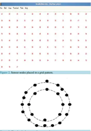
Figure 2 shows the placement of nodes in grid manner, the same simulation area as that of random network is taken with 100 nodes and all the nodes are held at a uniform distance. Going through most of the research papers, where for any application nodes are just deployed randomly. The main intention of the work is to give optimized positions for the nodes stating that the nodes are intended to work from the stated position till the node dies, therefore the developed algorithm will initially fix the position of nodes then go for the routing. Improved place- ment can definitely leads to effective utilization of network like routing, energy, co-ordination to give increased network lifetime.

Figure 3 shows the circular deployment of nodes which provides mainly two objectives. First one is, careful node placement can be a very effective optimization means for achieving the desired design goals, and is classi-fied as static approaches. On the other hand, some schemes have advocated dynamic adjustment of node loca-tion, since the optimality of the initial positions may become void during the operation of the network depending

Figure 2. Sensor nodes placed in a grid pattern.

on the network state and various external factors, We categorize the placement strategies into static and dynamic depending on whether the optimization is performed at the time of deployment or while the network is opera-tional, this approach considers positions of node metrics that are independent of the network state or assume a fixed network operation pattern that stays unchanged throughout the lifetime of the network.

To do the routing be it for all the 3 different node topology, a simple shortest path from a set of multipath from source and destination is been considered, the area considered for simulation is 100 × 100 m, in Figure 1

nodes are hardly distributed in a region of 50 × 50 m. The random deployment pattern indicates that nodes are densely deployed in one particular area, leaving behind most of the region uncovered. The proposed model con-siders a pattern of node distribution in grid and circular pattern in a way that for the grid it is with node at regu-lar intervals and for the circuregu-lar base station is located at the center surrounding a first layer of 8 sensor nodes covering equal area on a circle, followed by covering rest of the area on same pattern of deploying the nodes on a circular area so as to cover the complete simulation area. The advantage of optimized placement of node is that maximum area is covered; burden on nodes is reduced followed by increasing the network lifetime.

3.1. Mathematical Model

TheWSN which uses a method of random deployment of nodes can typically be replaced by uniform distribu-tion of nodes, be it in terms of grid or circular pattern of deployment of nodes. The work mainly concentrates on running a simulation using uniform node placement topology in a network, which is mainly worked for reducing the overall energy consumed by the network further increasing the network lifetime. Work is carried out consi-dering three different network topology in which sensor nodes are placed at different positions, the routing is held at different instant in the network based on which the energy consumption can be found. The methodology is as follows, considering a random distribution of sensor network, as the name suggests randomness, the nodes are placed at un-equal distance at different positions as shown in Figure 1. It can be seen from the Figure 1 that the nodes do not exhibit optimized location with randomness in x and y position, i.e. the two different nodes are never at equidistance. One of the important factor to consider is that, energy consumption depends on the dis-tance the data is been transmitted to reach the destination. This is an important consideration for WSN. One of the examples for uniform network can be grid based network as shown in Figure 2, here the node topology is at uniform distance forming a grid pattern. The network is defined in (100 × 100) distance. Each node is placed at a uniform distance of 1 m, considering the total number of nodes to be 100. Noting that network is scalable to distribute the nodes at an equal distance, varying the nodes from 0 to 99. The neighbor of any node can be at a distance of only 1m, which we call it as a uniform pattern of nodes. Let “n” be total number of nodes in a net-work choosing “n” equal to 100, then the total number of grids “k” that can be required, can be found by the following equation,

(

)

1

k= n− (1) where “k” be a number of grids

Let “d” be the distance between two nodes in a network and “R” be the radius within which, all the nodes are placed. The sensing range Rsense for a particular network can be given by,

2 sense

πR R

n

= (2)

The concept is based on the fact that nodes are predetermined. This can result in many advantages, especially when the node is replicated of energy, a particular node can easily be found and replaced. Hence the node loca-tion “NL” of every node in a network is given by,

sense

R NL

n

α =

× (3)

α

node which we call it as an optimized position of every node, which also holds good for circular placement of node topology. Another methodology for uniform node distribution can be a circular pattern of sensor nodes. The WSN in circular node placement topology is as shown in Figure 3. For simplicity circular deployment pat-tern of nodes is defined using two circles, here we have two types of communication. The data can be transmit-ted on a trajectory path or on circular path i.e. routing can go in both the paths depending on which the distance is shorter. Distance between the nodes for either of the methods is going to be varied. The trajectory method on trajectory path follows a distance of 1m between the neighbors, where the distance between the neighboring nodes are different for different circles. For the first circle it can be 0.39 m where 8 nodes are placed, for the second circle it is 1.56 m, by placing 16 nodes, and for the third circle it can be 3.51 m, for the fourth circle it can be 6.24 m. These distances can rather be called as “sectorial separation” which is given by,

2

1 π

sector

2 θ 180 r

   

=_ × ×_{ }× _

 

   (4)

r = a radius of a circle, θ be a angular difference between the nodes.

As with the uniform grid distribution pattern, node location is known for every node and it is not a random. Node locations are defined, where every node is placed on the on these locations, which is given by NLo

( )

o

NL =F

α

( )

= (6)

α

( )

α

Once the nodes are deployed on a circle, the routing can be done by any means, that is routing can be on a trajectory path or it can be on a circular path or both. Definiteness can occur as the nodes are again at uniformity. Once the different types of patterns are set, each node can be assigned with energy, traffic, neighbor identity and their energy. i.e. each node is assigned with 50 J of initial energy “Eini”. The time it transmits the data, there is

reduction in its total energy of a node that depends on the distance and traffic it carries on the path of its routing. Once the network is set up, data in terms of packet can be sent from source to the destination. One general method that we follow for 3 different networks node deployment is that, source and destination are chosen on the edges and with same positions then the routing is done. For the routing simple technique that we adopted is multipath based routing, where multiple routes from source and destination have been chosen. Path based on distance, neighbor, and traffic have been selected for routing. Once the routing takes place, the energy consumed by the network nodes is found, that is related to the network lifetime, the overall energy consumed from a par-ticular path between source and destination is given by “Etotal”

total 1 s i i E E =

=

∑

i = be the number of neighbors, s = total number of nodes, where Ei is given by,

1 1 j i n i k j k E e ′ = =

=

∑∑

ek is the energy consumption over the path of routing where data is been transmitted, n'—be the number of

nodes in the path, ij be number of hops, therefore ek is given by “ek”

k tx rec res

e =e +e +E (9)

etx anderec are transmission and reception energy constants for every hop, the mathematical model is been

de-veloped to find out the energy consumption (Eres) by the nodes during the routing using different deployment

pattern of nodes.

All the nodes are initially assigned with 50 J of energy say Eini which we call it as initial energy of a network

(Eini). A sensor consumes Esur = 50 nJ for transmitting unit of data and k = 100 pJ/bit/m2for the transmitting

am-plifier. So the energy consumption of sensor node in order to be active in the network is given by “Esur”

sur ene

As the energy consumed depends on the number of bits transmitted and hence if sensor node transmits K bits, then energy consumed in order to be active in the network is given by “Es(Actual)”

(

)

s ene

E = ×K E (11) At the destination nodes will receive packets, practically the received packets are less than actual packet sent. Hence energy consumed for receiving packets “Er(Actual)” is given by, which is lesser than Es

(

)

(

)

(

)

r p l

E = T −P (12) where Tp is the energy due to transmission and Pl is the energy lost due to packet loss.

Energy consumption of sensor Si in transmitting a unit of data packet to neighboring nodes “Enr”is given by (Actual) 2

0

n

nr r n I tr

n

E E n E d

=

=

∑

where nn is the number of neighoubrs, EI is the energy of each node and dtr is the distance of each neighbor from

source node.

The neighboring node is always with the burden to deliver the data to the destination node, the energy con-sumption of it turns out to be an important factor, which is calculated as “Er”

(Actual)

(

(

)

)

r r I n n tr

E =E +E n − n − d (14) Total energy consumed in network “Et”

t nr r

E =E +E (15) If there are “n” no of sensor nodes in a coverage area which are active and transmitting data, then total energy is,

tot t

E =nE (16) Residual energy for the sensor node is given by “Ere”

re ini t

E =E −E (17)

3.2. Lifetime Definition

We assume each node has the same initial battery energy Eo, the lifetime Tiof node Si is defined as the expected

time for the battery energy to be exhausted, given by “T(n)”

( )n k 100 ini

e T

E

= × (18)

where, n = number of sensor node. Taken with 100 to get the numerical in percentage.

Based on the energy model algorithm, simulation is been considered and comparative results are obtained for the pattern of nodes. Trajectory based node placement definitely saves the energy compared to random place-ment of nodes as shown in the below graphs.

4. Simulation

cal-culated using the mathematical model. Thus we find out residual energy of the network after the routing takes place. The wireless sensor network is considered to be static, following inputs are considered for simulation. Number of nodes = 100, Initial energy of each node is 50 J, Eele = 50 nJ/bit/threshold distance, radio dissipation of transmitter and receiver Eamp = 100 pJ/bit/m^2, Communication range = 20 units. Simulation is to generate WSN topology, byapplying AODV routing protocol algorithm to each topology, then calculating the energy, lifetime, hops that are performance parameter of the network.

The Performance parameters measured are as follows.

• Intermediate Nodes: It is the number of hops (nodes) required to transmit data from source to destination

• Residual Energy: The amount of energy that remains after the routing during data transfer

• Network Lifetime: It is the ratio indicating the utilization of total life of the network in transmitting the data The result of simulation demonstrates that, initial deployment of node topology is considered by placing node on a uniform path, the energy consumption of each node and total network energy consumption is considered and compared with the random node placement pattern. The result that is shown proves that energy consumption is definitely less with grid deployment having distributed the node in whole of the simulation area, where as random placement tries to cover only half of the simulation area, following which the algorithm tries to save the energy consumed by the network, covering maximum area with increase in lifetime of network.

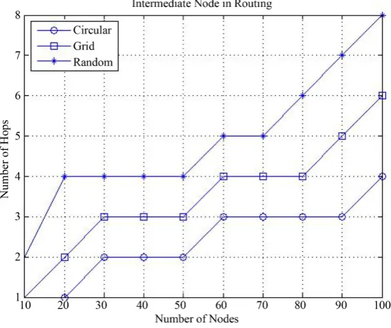
Figure 4 shows number of intermediate nodes or hops that are used to transmit the data between two ends, the results shows that it is based on the definiteness of the node position as the grid and circular network nodes use maximum communication radius for finding the next hop. The number of hops required to reach the destination in uniform network are definitely less as compared with random network as with the simulation results. The

Figure 5 gives the amount residual energy saved by the random, circular, grid based topologies that are calcu-lated after the routing is been carried out. It is shown from Figure 5 that random network consumes the highest amount energy for the routing. Figure 6 gives the network lifetime that relates to usage of a network from the consumed energy. From the graph we can conclude that random based topology network lifetime is less com-pared to other two topologies. The simulations are done for a single routing, i.e. considering the part of data that is transmitted in one round of routing, when such 1000 rounds are considered for routing it is definite that ener-gy as network parameter would definitely add to improve the performance of a network.

5. Conclusion

The work is carried to simulate the sensor network, to differentiate the behavior of network under different

Figure 5. Graph showing residual energy in joules vs number of nodes.

Figure 6. Showing graph of percentage of network lifetime vs number of

nodes.

References

[1] Biradar, R.V., Patil, V.C., Sawant, S.R. and Mudholkar, R.R. (2012) Classification and Comparision of Routing Pro-tocol in Wireless Sensor Network. Journal of Special Issue on Ubiquitous Computing Security Systems, 4, 704-711. [2] Rupam, P.D. (2014) Analysis of Routing Protocols on Wireless Sensor Network: A Survey. International Journal of

Advanced Computational Engineering and Networking, 2.

[3] Roseline, R.A. and Sumathi, P. (2011) Energy Efficient Routing Protocols and Algorithms for Wireless Sensor Net-works—A Survey. Global Journal of Computer Science and Technology, 11.

[4] Singh, S.K., Singh, M.P. and Singh, D.K. (2010) Routing Protocols in Wireless Sensor Networks—A Survey. Interna-tional Journal of Computer Science & Engineering Survey (IJCSES), 1.

[5] Hojjatoleslami, S., Aghazarian, V. and Aliabadi, A. (2011) DE Based Node Placement Optimization for Wireless Sen-sor Networks. 3rd International Workshop on Intelligent Systems and Applications (ISA), 1-4.

[6] Tian, H., Shen, H. and Roughan, M. (2008) Maximizing Networking Lifetime in Wireless Sensor Networks with Reg-ular Topologies. Ninth International Conference on Parallel and Distributed Computing, Applications and Technolo-gies, Otago, 1-4 December 2008,211-217. http://dx.doi.org/10.1109/pdcat.2008.29

[7] Cheng, P., Chuah, C.-N. and Liu, X. (2004) Energy-Aware Node Placement in Wireless Sensor Networks. Global Tel-ecommunications Conference, 2004. GLOBECOM '04. IEEE, 5, 3210-3214.

[8] Lam, M.-L. and Liu, Y.-H. (2006) Active Sensor Network Deployment and Coverage Enhancement Using Circle Packings. IEEE International Conference onRobotics and Biomimetics,2006. ROBIO '06,Kunming, 17-20 December 2006, 520-525.

[9] Gun, M., Kosar, R. and Ersoy, C. (2007) Lifetime Optimization Using Variable Battery Capacities and Nonuniform Density Deployment in Wireless Sensor Networks. 22nd international symposium on Computer and Information Sciences,2007. ISCIS 2007, 7-9 November 2007, 1-6.

[10] Liang, W.F., Ma, G.J., Xu, Y.L. and Shi, J.G. (2008) Aggregate Node Placements in Sensor Networks.11th IEEE Sin-gapore International Conference onCommunication Systems, 2008. ICCS 2008,Guangzhou, 19-21 November 2008, 926-932. http://dx.doi.org/10.1109/iccs.2008.4737320

[11] Zhang, J., Ci, S., Sharif, H. and Alahmad, M. (2009) Lifetime Optimization for Wireless Sensor Networks Using the Nonlinear Battery Current Effect. IEEE International Conference onCommunications, 2009. ICC’ 09,Dresden, 14-18 June 2009, 1-6. http://dx.doi.org/10.1109/icc.2009.5199132

[12] Tariq, M., Kim, Y.-P., Kim, J.H., Park, Y.-J. and Jung, E.H. (2009) Energy Efficient and Reliable Routing Scheme for Wireless Sensor Networks. International Conference on Communication Software and Networks, 2009. ICCSN’ 09, Macau, 27-28 February 2009, 181-185.http://dx.doi.org/10.1109/iccsn.2009.101

[13] Malik, N.N.N.A., Esa, M. and Yusof, S.K.S. (2009) Intelligent Optimization of Node Coordination in Wireless Sensor Network. Innovative Technologies in Intelligent Systems and Industrial Applications, 2009. CITISIA 2009,Monash, 25-26 July 2009, 328-331.

[14] Li, W. (2009) Wireless Sensor Network Placement Algorithm. 5th International Conference onWireless Communica-tions, Networking and Mobile Computing, 2009. WiCom’ 09, Beijing, 24-26 September 2009, 1-4.

[15] Botros, S.S., Elsayed, H.M., Amer, H.H. and El-Soudani, M.S. (2009) Lifetime Optimization in Hierarchical Wireless Sensor Networks. IEEE Conference onEmerging Technologies & Factory Automation, 2009. ETFA 2009, Mallorca, 22-25 September 2009, 1-8. http://dx.doi.org/10.1109/etfa.2009.5347016

[16] Nik Abd Malik, N.N., Esa, M. and Yusof, S.K.S. (2009) Optimization of Adaptive Linear Sensor Node Array in Wire-less Sensor Network. Asia Pacific Microwave Conference, 2009. APMC 2009, Singapore, 7-10 December 2009, 2336- 2339. http://dx.doi.org/10.1109/apmc.2009.5385453

[17] Abbasy, M.B., Barrantes, G. and Marín, G. (2010) Performance Analysis of Sensor Placement Strategies on a Wireless Sensor Network. 20104th International Conference onSensor Technologies and Applications (SENSORCOMM), Ve-nice, 18-25 July 2010, 609-617. http://dx.doi.org/10.1109/SENSORCOMM.2010.96

[18] Akshay, N., Kumar, M.P., Harish, B. and Dhanorkar, S. (2010) An Efficient Approach for Sensor Deployments in Wireless Sensor Network. 2010 International Conference on Emerging Trends in Robotics and Communication Tech-nologies (INTERACT),Chennai, 3-5 December 2010, 350-355. http://dx.doi.org/10.1109/interact.2010.5706178 [19] Li, X. and Qiu, S.B. (2011) Research on Multicast Routing Protocol in Wireless Sensor Network. International

Confe-rence onControl, Automation and Systems Engineering (CASE), Singapore, 30-31 July 2011, 1-4.

http://dx.doi.org/10.1109/iccase.2011.5997642