Reconstruction of Temporal Images by Gradient
based Sequential Prediction
Boshir Ahmed
Department of Computer
Science & Engineering,
Rajshahi University of
Engineering & Technology,
Bangladesh
Md. Al Mamun
Department of Computer
Science & Engineering,
Rajshahi University of
Engineering & Technology,
Bangladesh
Md. Mortuza Ali
Department of Electrical &
Electronic Engineering,
Rajshahi University of
Engineering & Technology,
Bangladesh
ABSTRACT
The identification of the factors involved in change detection could lead to a comprehensive understanding of real changes and non-real changes on a broad scale, as well as prediction capability. As a huge amount of remotely sensed data is available, most of the applications require the interpretation of images collected over a period. Frequently collected satellite images mostly present strong spatial redundancies for real changes such as deforestation, urbanization, flood, bushfire etc. and non-real changes due to various system factors or environmental noise such as illumination variation and atmospheric effects. In this case, the pixel values of two images are not same. Therefore nonlinear regression prediction model such as gradient adjusted temporal prediction procedure is applied to predict a temporal image for detecting the types of changes have occurred and is presented in this paper. As the changes are detected iteratively, the whole process converges towards the final model that better defines the temporal correlation between two adjacent images.
Keywords
Gradient adjusted temporal prediction, temporal correlation, real and non-real changes.
1.
INTRODUCTION
Change detection from satellite images is important for some applications including urban planning, environmental monitoring and hazard detection[1]. The satellite images are often affected by sensor, illumination variation, atmospheric absorption and other environmental effects. The changes may be happened by deforestation, urbanization; and most of these changes are gradual or incremental [2]. Generally, the neighbouring pixels should have similar values, so a pixel can still be predicted from its neighbours. The pixels can be predicted because the images exhibit high temporal correlation. However, abruptly changed pixels do not follow this.
A wide variety of change detection methods have been developed in the remote sensing literature [1, 3]. Most commonly used change detection techniques are principal component analysis, post-classification comparison and change vector analysis [4, 5, 6, 7]. The principal component analysis showed a poor performance when the images are weakly correlated [8, 9]. The real changed pixels are difficult to predict from the previous reference image because they are mixed with system’s noise. Applying de-correlation through single model regression to the affected pixels lead to a good
approximation of those pixels. But large errors/residual can occur in the case of real changed pixels which do not follow that model. If real or non-real changes are taken place then the neighbouring pixels do not comply the similar values. The input images will provide low correlation among them due to many land-cover changes. In such cases the input data will be non-linearly related [2]. Therefore in this paper, nonlinear regression prediction model based on median edge detection (MED) and gradient adjusted temporal prediction method is proposed to predict the current image from the previous image. The prediction of the data set is completely on how well the pixels are correlated. Therefore spatial correlation measure is incorporated to determine the order of prediction [2, 4]. As the changes are removed, the whole process converges towards the final model that better define the spatial relationship between the pixels. Experimental results demonstrate that the proposed method is effective, especially when the new data are not highly correlated to the previous data.
2.
METHODOLOGY
Satellite images are highly spatially correlated because the neighbouring pixels are homogenous in nature. The correlation value reduces only around the edges for abrupt value transition. So any pixels can be predicted from neighbouring pixels by non-linear regression [4]. The principal premise which justifies the use of non-linear regression for spatial predictions. If real changed pixels in temporal images are considered as nonlinear components, the nonlinear predictor is expected to give a better performance. When proposed method applied appropriately on the images having minor real changes, it is able to provide prediction results close to linear prediction.
As the correlation can measure the linear dependency between two images, the temporal correlation of two images can be utilized to determine the types of changes (real change or non-real change).
2.1
Temporal Correlation
Salient property of remote sensing satellite images is that high spectral correlation exists among the spectral bands. The correlation coefficient measures the strength of the linear association between variables and quantifies. The correlation coefficient between two data sets
X
[
x
i]
and Y=[yi] , is
n i n i i i n i i i XYy
y
x
x
y
y
x
x
r
1 1 2 2 1)
(
)
(
)
)(
(
(1)where
x
andy
are the sample means ofX
and Y, respectively and n is the total number of pixels. Although linear regression and correlation are related but it cannot find the best-fit line [10]. However, the regression function can be chosen according to the relationship indicated by the spatial correlation.2.2
Prediction
It is assumed that, for a fixed value in the previous image,
i
x
X
, the values in the current image are listed as}
{
y
jY
. Here,i
,
j
1
,...,
m
are the numbers of occurred grey levels for the input images. For multi-spectral images, the predicted value of each gray levelx
i, is calculated as,
m j j ji
w
y
y
1(2)
where the weight factor,
w
, depends on the conditionaldensity of [Y] given that the values of
x
i and the predictedvalue is actually the mean of the conditional density of
y
jgiven
x
i.2.3
Non Linear Prediction
Non-linear predictors are suited for their adaptive ability in prediction. Most of them are classified as switching predictors based on their local features. The Median Edge Detector (MED) predicts a pixel depending on the edges around it. If the real changed pixels in the temporal images are considered as non-linear components, the non-linear predictor is expected to give a better performance. Here non-linear function is used to predict the current image from the previous image and is defined as:
p p
x
x
x
0
1 1
2 2
...
...
(3)where λ is a non-linear polynomial function and p is the degree of the polynomial.
[image:2.595.57.209.75.141.2]2.3.1Gradient Adjusted Temporal Prediction
The horizontal and vertical edges can be identified according to some given condition when applied to the neighbourhood pixels and prediction of current pixel is obtained by assigning its values to the pixels which are not part of the edges (Fig. 1). If there is no edge, the predicted pixel is on the plane defined by the three neighbouring pixels. The conditions for detecting the edges are given below.Fig 1: MED predictions by edge detection
1.
if
x
(
i
1
,
j
1
)
max
x
(
i
,
j
1
),
x
(
i
1
,
j
)
then predictedx
(
i
,
j
)
min
x
(
i
,
j
1
),
x
(
i
1
,
j
)
2.
if
x
(
i
1
,
j
1
)
min
x
(
i
,
j
1
),
x
(
i
1
,
j
)
then predictedx
(
i
,
j
)
max
x
(
i
,
j
1
),
x
(
i
1
,
j
)
3. otherwise, predicted
)
1
,
1
(
)
,
1
(
)
1
,
(
)
,
(
i
j
x
i
j
x
i
j
x
i
j
x
This idea can also be extended to temporal prediction. If an edge is detected at the current location in previous image, it is highly likely to occur in the current image. In a related prediction approach, the prediction of the current pixel in the current image is accomplished by considering the local gradients [11]. Considering the neighborhood from the previous image and the current image in Fig 2, the gradient-adjusted temporal predictor can be given by the following conditions.
(a) (b)
Fig 2: (a) Pixels’ neighbourhoods in previous reference image, (b) current image.
Overall Procedure
The steps of the overall process are detailed below.
1. Predict the current image,Y, from the previous image,
X
, by gradient adjusted temporal prediction using the following conditions .
if
x
(
i
,
j
)
x
(
i
1
,
j
)
|
|
x
(
i
,
j
)
x
(
i
,
j
1
)
T
then predicted
)}
1
,
(
)
,
(
{
)
1
,
(
)
,
(
i
j
y
i
j
x
i
j
x
i
j
p
elseif
x
(
i
,
j
)
x
(
i
1
,
j
)
|
|
x
(
i
,
j
)
x
(
i
,
j
1
)
T
then predicted
)}
,
1
(
)
,
(
{
)
,
1
(
)
,
(
i
j
y
i
j
x
i
j
x
i
j
p
otherwise
predicted2 )} 1 , ( ) , ( { ) 1 , ( )} , 1 ( ) , ( { ) , 1 ( ) ,
(i j yi j xi j xi j yi j xi j xi j
p
where T is a threshold and
is selected globally by running linear regression between the two images. The first condition identifies the sharp horizontal edge and the second the sharp vertical edge. Similarly, temporal gradient can be calculated between the two images and suitable predictors can also be designed for adaptive prediction. [image:2.595.320.560.350.428.2]5. Then, trim the imaged data,
x
i andy
i, as follows:
if
(
p
(
x
i)
y
i
T
1)
,remove
x
i from Xandy
i from Y; and the trimmeddata for the next step, kth regression becomes X=
x
ikand Y=
y
ik.6. Run the regression again on
x
ikandy
ikand then updatedregression function is
p
(
x
i)
a
kx
ik
k.7. If |
a
k-a
k1| > T2 , repeat steps (2) to (7).8. Find the residual, D, for all the pixels using the final model parameters.
9. Find the standard deviation SD of D.
10.Pixels values of D which are greater than n× SD are set to value 0 and the rest are set to 1, where n are selected by trial and error procedure by matching with the current image. The resultant mask indicates the location of the changes.
T2 is a very small value which indicates the negligible amount
of change between the
a
values in successive iteration. The number of iterations required depends on the difference between the percentages of estimated and the percentage of the changes contained in the current image.3.
EXPERIMENTAL RESULTS
[image:3.595.315.543.72.236.2]In non-linear prediction the threshold value might be changed to predict the temporal changed pixels. If threshold values are increased gradually, the correlation of the current and the predicted images will also be increased. This indicates that the higher threshold, lead the prediction toward the accurate result. Table 1 shows the gradual increase in correlation values with increasing threshold value. This is shown in graphically in Fig. 3
Table 1. Incremental correlation value with gradual increase in threshold value
Threshold Correlation Value (10-2)
0 95.89228182
10 96.12816329
20 96.27880336
30 96.37969851
40 96.47166139
50 96.53732413
60 96.59213699
70 96.62547013
80 96.65616551
[image:3.595.326.523.329.734.2]90 96.67873702
Fig 3: Correlation Vs Threshold
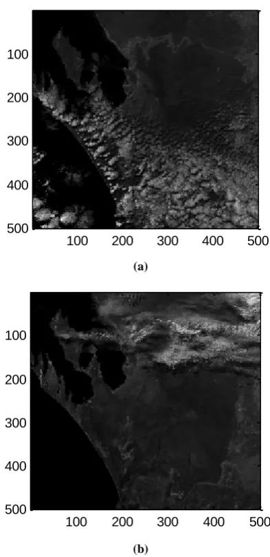
The proposed algorithm was applied to a Moderate-resolution Imaging Spectroradiometer (MODIS) image captured on a part of Western Australian and it is shown in Fig.4. In the experiment only the image band 1 was used to avoid the processing difficulty and the predicted image is shown in Fig.5
(a)
(b)
Fig 4: MODIS image used for the experiment (Courtesy: GeoScience Australia) (a) Previous Image, (b) Current
Image
95.8
96
96.2
96.4
96.6
96.8
0
50
100
C
o
rr
el
at
io
n
Threshold
100 200 300 400 500 100
200
300
400
500
100 200 300 400 500 100
200
300
400
[image:3.595.56.278.502.691.2]Fig 5: Temporal correlation between two adjacent images
[image:4.595.322.527.104.503.2]The temporal correlation of the current and the previous image is shown in Fig 5 and it can be seen that the measured correlation does not provide a liner relationship. Therefore, nonlinear prediction method is applied and the resultant image is shown in Fig 6.
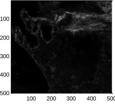
Fig 6: Predicted image of current image
Fig 7: Residual image after median filtering
From the current and previous image the residual image is determined and is shown in Fig 7 after median filtering.
After masking the subtracted absolute value of the current image from predicted image, the resultant image indicates the changed location and it is shown in Fig 8.
(a)
[image:4.595.67.258.321.495.2](b)
Fig 8: Detecting Changes, (a) Real Change, (b) Non-real Change
4.
CONCLUSION
An algorithm for determining the change detection of two adjacent images based on Median Edge Detection (MED) and the gradient adjusted temporal prediction (GATP) is proposed. The proposed method identifies the spatial edges of the reference image by gradient analysis which makes the predicted image good resembles of the actual scene by removing the unwanted errors. In this purpose temporal gradient can be calculated between the two images and suitable temporal gradient-adjusted predictors can also be designed for adaptive temporal prediction.
5.
FUTURE RESEARCH DESCRIPTION
The lack of resemblance between the pixels of two dates’ images can cause large errors in temporal prediction. This difference can be due to geometric distortion or radiometric errors. Therefore, high-quality image registration and radiometric correction are the pre-requisites for achieving high prediction gains. Additional research into geometric error rectification and radiometric correction will be valuable for making temporal prediction more effective.
0 50 100 150 200 250
-0.6 -0.4 -0.2 0 0.2 0.4 0.6 0.8 1
Blocks
T
e
m
p
o
ra
l
C
o
rr
e
la
ti
o
n
100 200 300 400 500 100
200
300
400
500
100 200 300 400 500 100
200
300
400
500
100 200 300 400 500 100
200
300
400
500
100 200 300 400 500
100
200
300
400
[image:4.595.68.260.538.714.2]6.
REFERENCES
[1] A. Singh, “Digital change detection techniques using remotely sense data.” International Journal of Remote sensing, vol. 10,No.6, 989-1003, (1989).
[2] Penna, B., Tillo, T., Magli, E., and Olmo, G. “Hyperspectral Image Compression Employing Model of Anomalous Pixels.” IEEE Geoscience and Remote Sensing Letter, vol 4, No 4, 664-668, (2007)
[3] Tian, M., Wan, S., and Yue, L. " A Novel Approach for Change Detection in Remote Sensing Image based on Saliency Map." Proceeding of the 4th International Conference on Computer Graphics, Imaging and Visualization (CGIV '07), 397-402, (2007).
[4] Motulsky, H., and Christopoulos, “Fitting Models to Biological Data Using Linear and Nonlinear Regression: A Practial Guide to curve Fitting”. Oxford University Press.
[5] Radke, R. J., Andra, S., Al-Kofahi, O., and Roysam, B. "Image change detection algorithms: a systematic survey." IEEE Transactions on Image Processing, 294-307,(2005).
[6] Torma, M., Harma, P., and Jarvenpaa, E. "Change detection using spatial data problems and challenges."
IEEE International Geoscience and Remote Sensing Symposium (IGARSS '07), 1947-1950, (2007). [7] Bruzzone, L., and Prieto, D. F. "Automatic analysis of the
difference image for unsupervised change detection." IEEE Transactions on Geoscience and Remote Sensing, vol.38, No.3, 1171-1182, (2000).
[8] Qiu, B., Prinet, V., Perrier, E., and Monga, O."Multi-block PCA method for image change detection." 12th International Conference on Image Analysis and Processing, 385-390, (2003)
[9] Fauvel, M., Chanussot, J., Benediktsson, J., and Atli, n. "Kernel Principal Component Analysis for the Classification of Hyperspectral Remote Sensing Data over Urban Areas." EURASIP Journal on Advances in Signal Processing, 1-14, (2009).
[10] Weinberger, M.J., Seroussi, G., and Sapiro, G. “The LOCO-I lossless image compression algorithm: principles and standardization into JPEG-LS.” IEEE Transactions on Image Processing, vol 9 No. 8, 1309-1324, (2000).