Commercial and Industrial Demand Response
Under Mandatory Time-of-Use Electricity
Pricing
∗Katrina Jessoe†
David Rapson‡
This paper is the first to evaluate the impact of a large-scale field deployment of mandatory time-of-use (TOU) pricing on the energy use of commercial and industrial firms. The regulation imposes higher prices during hours when electricity is generally more expensive to produce. We exploit a natural experiment that arises from the rules governing the program to present evidence that TOU pricing induced negligible change in overall usage, peak usage or peak load. As such, economic efficiency was not increased. Bill levels and volatility exhibit minor shifts, suggesting that concerns about increased expen-diture and customer risk exposure have been overstated. JEL: D22, L50, L94, Q41
Keywords: Regulation; Electricity; Time-of-Use
Pric-ing.
∗We thank, without implicating, Lucas Davis, Kenneth Gillingham,
Koichiro Ito, Chris Knittel, Aaron Smith and Jeffrey Williams. Thanks also to United Illuminating personnel for assistance in obtaining the data and shedding light on institutional details. Comments from seminar par-ticipants at AERE, RFF, Stanford, the UC Energy Institute, UCE3 and U. Melbourne helped to improve this draft. Tom Blake and Brock Smith provided excellent research assistance. We also thank the University of California Center for Environmental and Energy Economics (UCE3) for fi-nancial support. Rapson thanks the Energy Institute at Haas for support under a research contract from the California Energy Commission. All errors are our own.
†Department of Agricultural Economics, University of California,
Davis, One Shields Ave, Davis, CA 95616; Phone: (530) 752-6977; Email: kkjessoe@ucdavis.edu
‡Department of Economics, University of California, Davis, One
Shields Ave, Davis, CA 95616; Phone: (530) 752-5368; Email: dsrap-son@ucdavis.edu
I INTRODUCTION
In the electricity market, marginal costs vary by the minute but retail prices are (for the most part) time-invariant. Because of this, the market does not function efficiently and substantial economic loss may result, both in the short-run and the
long-run.1 The disparity between wholesale and retail prices leads to
chronic over- and under-consumption at different times of the day, excess capital investment to prevent blackouts, and an in-crease in the opportunity for fringe producers to exploit market power. Estimates place the magnitude of the deadweight loss from time-invariant retail electricity prices in the tens of billions
of dollars annually in the U.S.2 The clear first-best policy would
be a retail price which varies to reflect real-time fluctuations in the wholesale market. However, technological and political obstacles have forced regulators to proceed with caution, and, if deviating from flat-rates at all, implement a coarse variant of time-varying incentives called ‘time-of-use’ (TOU) pricing. This study documents evidence from one deployment of TOU pricing in the field for commercial and industrial (C&I) customers.
TOU pricing is the most common incentive-based tariff that is currently implemented by utilities and regulators to address peak load challenges. Under this tariff, two (sometimes three) periods each day are designated as high, medium or low demand according to historic patterns, and higher prices are assigned to higher-demand hours. One potential implementation of TOU is
illustrated in Figure??. In this scenario, peak hours are defined
as occurring between 10am - 6pm. ‘Peak usage’ (measured in kilowatt-hours, or kWh) is the cumulative amount of electricity used during that period of time, and ‘peak load’ (measured in kilowatts, or kW) is defined as the maximum throughput at any
moment during the course of a month.3 Under TOU pricing,
customers incur a higher charge for peak usage (kWh) that oc-curs between the peak hours of 10am - 6pm, and a lower charge 1During the California energy crisis in 2001, wholesale electricity prices
exceeded $1,400 per mWh, or $1.40 per kWh, more than twenty times the then retail price of $0.067 per kWh.
2Borenstein & Holland [2005] estimate that 5-10 percent of the market
is deadweight loss. In 2009, $350 billion worth of electricity was consumed in the United States, implying an annual inefficiency on the order of $17 - $35 billion, roughly 2-3 times the entire budget of the Environmental Protection Agency (just over $10 billion in 2010).
3Note that, for simplicity, Figure??displays just one day, but the same
for usage that occurs during off-peak hours.
Place Figure ?? About Here
The intention of the TOU tariff is to induce consumers to change their behavior by reducing demand during peak hours, potentially by shifting usage to off-peak hours. This rate struc-ture may be viewed as a either a regulatory ‘baby step’ towards dynamic pricing or a pragmatic compromise, depending on one’s perspective. A perceived advantage of this rate structure over more granular versions (e.g. critical-peak pricing or real-time pricing) is that customers can readily understand it and, in the-ory, respond to it. Its fundamental drawback is coarseness; TOU pricing as currently devised can capture no more than 6
per-cent of wholesale market price variation in Connecticut.4 Given
this upper bound, it is important to understand whether TOU pricing achieves the goal of reducing peak demand. If it does not, then either it should be replaced by a more effective pol-icy (potentially a more granular and timely polpol-icy, like real-time pricing), or regulators should clearly state that TOU is intended as a transitional strategy on the path to such a policy. In this paper we present quantitative evidence that the response to a large-scale field deployment of mandatory TOU pricing for C&I customers in Connecticut was minimal.
Our empirical setting has several attributes that make it attractive for evaluating TOU pricing. First, TOU pricing is assigned to some firms via a quasi-random mechanism. The mandatory TOU assignment rule states that C&I firms whose peak load breaches a pre-determined threshold are placed on a TOU schedule and cannot, regardless of future behavior, re-turn to a flat-rate tariff. While firms can influence peak load, they cannot control it precisely. Thus, in the neighborhood of the threshold, status as a ‘crosser’ is plausibly random and the setting lends itself to a regression discontinuity design.
A nuance of our setting is that in the years preceding the mandatory TOU policy, firms had the option to select onto the TOU rate. This does not impact the validity of our results, and in fact provides regulators and policy makers with results from the most relevant setting. If other utilities introduce mandatory 4Borenstein [2005] performs similar calculations for California and New
Jersey, and estimates that 6 to 13 percent of wholesale market variation is captured by TOU pricing.
TOU pricing, as is being considered universally in the US today, it is certain to be accompanied by a voluntary adoption mech-anism. Thus it is not a coincidence that our setting shares the most important features of potential future deployments being considered by policymakers in other jurisdictions.
A second feature of our empirical setting is that firms as-signed to treatment are exposed to exogenous variation in prices. We observe (roughly) two draws from the menu of potential prices. One is the time-invariant rate that ‘control’ firms in-cur throughout the period of study, and the other is the TOU rate schedule imposed on ‘treatment’ firms. In our setting, as-signment to treatment involves three price changes: the kW peak-load charge decreases, and the previously time-invariant kWh charge increases during peak hours and decreases during off-peak hours. We will discuss the incentives that these price changes generate in Section 2. Since the price schedule was pro-duced by an actual rate determination process, we view it as the most relevant of the potential rates in our setting. However, it is reasonable to expect that rates transmitting different incentives would produce different results. As such, our estimates of the customer response should be viewed as a single realization from this distribution. The near impossibility of observing a broad menu of price alternatives in a single field setting highlights the need for multiple peer-reviewed studies on this topic. To our knowledge there has not been one in the US in nearly three decades (Aigner & Hirschberg [1985]).
Finally, our setting has cross-sectional and time-series varia-tion that allows us to account non-parametrically for important firm characteristics and aggregate demand shifters. We use a monthly panel dataset from the universe of customers in the utility’s ‘General Services’ rate class, allowing us to exploit vari-ation both over time and across space to estimate the impact of this policy on usage, peak load and expenditure.
Our analysis yields four primary results. First, in the first year following assignment to mandatory TOU pricing, we can-not reject the hypothesis of no change in electricity usage be-havior. In our preferred specification, we can rule out aggregate decreases of greater than 2 percent in monthly consumption and peak load in response to treatment. Second, we find that, on average, firm electricity bills decrease. This is due to a rate-class discount implicit in the price schedule, rather than a behavioral response. After adjusting the analysis to account for the rate
class discount, TOU pricing does not impact monthly electricity expenditure (lending support to our lack of evidence of measur-able behavioral change). Third, a direct implication of the first two findings is that they restrict the feasible amount of load shifting that to around one percent of usage. Fourth, increases in bill levels and bill volatility are minimal, with only a small number of firms being adversely affected.
Our work contributes a new data point to the sparse em-pirical literature on C&I TOU pricing. Earlier evidence from electricity markets suggests that TOU pricing is at best mod-erately effective among C&I users (Aigner & Hirschberg [1985],
Aigner et al. [1994]).5 Using quasi-experimental data, Aigner
& Hirschberg [1985] find strong complementarity between peak and off-peak usage, and evidence of small but statistically sig-nificant substitution from peak to off-peak hours in response to TOU pricing. Their results also suggest that the magnitude of the differential between peak and off-peak prices influences re-sponse. Their setting is less than ideal due to the fact that par-ticipants, though randomly assigned to control and treatment, are allowed to opt out if adversely affected by the treatment. In a randomized controlled trial in Israel, Aigner et al. [1994] also detect small but significant shifts in usage by firms. In both experiments, the price change is explicitly temporary in nature. The permanence of TOU pricing in our setting is another feature that contributes to policy relevance.
Finally, our results shed light on the ongoing policy debate about whether TOU rates should be mandated or voluntarily implemented (if at all). Driven by concerns about excess harm from high bill levels or dramatic increases in bill volatility, most TOU tariffs in the U.S. have been introduced voluntarily, with
customers having the option to select into a TOU rate.6 Our
5A long empirical literature has also studied residential responsiveness
to time-variant electricity pricing, finding evidence that some policies in-duce a shift in peak to off-peak usage (Wolak [2007]) while others inin-duce conservation (Allcott [2010], Faruqui & Sergici [2011], and Jessoe & Rapson [forthcoming]). A review of residential dynamic pricing experiments can be found in Faruqui & Sergici [2010].
6In February 2010 the President of the California Small Business
As-sociation warned that ‘...with dynamic pricing, small businesses will send workers home, tell workers not to come into work or pay large electric bills for using power on peak days.’ In response, PG&E successfully petitioned to delay its TOU deployment, though it nonetheless launched in November 2012.
results suggest these concerns have been overstated. Of treated firms in our sample, 95 percent experience bill increases of less than 8.5 percent and bill volatility increases on average by less
than 5 percent.7
II INDUSTRY AND REGULATORY SETTING
A vast economic literature dating back a century has described the theoretical rationale for implementing time-variant retail electricity prices. Williamson [1966] constructs a welfare frame-work that reveals what is now common knowledge: that the so-cially optimal amount of generation capacity will require some form of rationing during periods of peak demand, and that it can be achieved by equating the retail price to short-run marginal cost. This observation has been repeated in subsequent years, generally during periods when turbulent electricity markets are disruptive enough to earn popular attention. One of the clearest expositions, in our view, is from Borenstein [2005].
The argument proceeds as follows. Demand is highly vari-able, supply faces strict constraints in the short run, and eco-nomically feasible storage at an industrial scale does not exist. In the event that demand exceeds supply, grid failure results in widespread ‘blackouts’. On the other hand, excess supply damages expensive equipment. An engineering challenge in this industry is thus the necessity of equating supply and demand in real time. When demand is low the grid operator simply deploys less generation capacity; but when demand rises, gen-eration facilities approach and then hit their capacity. At this point, either more marginal facilities must be brought online, or demand must be reduced in some way (often by implement-ing scheduled regional blackouts). The revealed preference in developed nations is to build sufficient excess capacity to cover demand during the peak hours. By implication, the marginal firms that are engaged in these few hours are unnecessary at all other times.
As it turns out, this situation results in large welfare losses due in large part to the time-invariant rates being charged to retail electricity customers. Marginal benefit equals marginal 7Even this is conservative, having been calculated using bill levels
al-ready adjusted for the TOU rate-class discount implicitly offered by the CT policy. In any case, high volatility could also be mitigated by the de-velopment and availability of simple hedging instruments, as suggested in Borenstein [forthcoming].
cost only by chance and for fleeting moments during the day or year, implying chronic over- or under-consumption with respect
to the social optimum. Generation is overbuilt as insurance
against blackouts. And marginal firms (even those with low market share) face a sharply inelastic demand curve, giving them the capability to exercise market power during hours of system
peak.8 The cumulative welfare loss due to these features of the
market have been estimated at approximately 5-10 percent of value in the wholesale electricity market (Borenstein & Holland [2005]).
These facts are not lost on regulators, and most economists acknowledge the importance of better understanding market
outcomes in this setting. In his work on peak load pricing,
Steiner [1957] laments ‘an almost total absence of empirical evi-dence as to the importance of the potential shifting peak...’. Re-cently with the proliferation of smart metering technology that allows electricity use to be measured at high frequency, there has been a renewed empirical focus on evaluating the potential of time-varying pricing. We add to this discussion by analyzing the first large-scale C&I field deployment of mandatory TOU.
In 2006, the Connecticut Department of Public Utilities and Control (DPUC) issued an order requiring United Illuminating (UI), an electric utility serving over 324,000 residential and C&I customers in Connecticut, to phase in mandatory TOU pric-ing for commercial users. This policy was approved and im-plemented in an effort to reduce growing demand for electricity during peak periods. In coordination with the DPUC, UI es-tablished peak load thresholds that, if exceeded, would cause a firm to be placed on mandatory time-of-use pricing. Once transferred onto the TOU tariff, a firm could not return to the
flat-rate schedule, regardless of future consumption.9 The first
two demand thresholds took effect on June 1, 2008 at 300kW and June 1, 2009 at 200kW. The majority of small commercial users did not approach either of these. However, on June 1, 2010 the threshold declined to 100kW, and a substantial number of users were switched to TOU rates as a result of having crossed 8This was a major cause of the California electricity crisis in 2000, as
described in Borenstein [2002].
9Firms could choose to purchase generation from an alternate supplier.
However, as shown in Table ?? the majority of the TOU price differen-tial is transmitted through distribution charges, which are charged to all customers, regardless of the generation supplier.
it.
Historically, small and medium-sized commercial users in UI’s territory paid a single rate per kilowatt-hour (kWh) re-gardless of when electricity was consumed, unless they opted
into TOU pricing.10 Since 1978, any general services customer
could select into TOU pricing in lieu of the flat-rate. Similar to mandatory TOU pricing, once customers volunteered for this tariff they could not return to the flat-rate schedule. Also, since the early 1980s, customers reaching peak load in excess of 500kW were mandated onto TOU pricing.
In our setting, customers that crossed the threshold were placed on a TOU tariff that charged a higher peak rate for elec-tricity consumed between 10am - 6pm on Monday-Friday, and a lower off-peak rate during all other hours. The incentive cre-ated by these two rate changes is to shift usage from peak to
off-peak hours. Table ?? reports the rate schedules in 2010 for
commercial customers on a flat-rate and TOU rate. For flat-rate customers the price per kWh of electricity is $0.1791 in the win-ter and $0.1842 in the summer. By comparison, TOU customers pay a higher price for electricity during peak hours, $0.2237 in the winter and $0.2364 in the summer, and a lower price dur-ing off-peak hours, $0.14391 in the both the summer and the winter. This amounts to between a 55 to 64 percent increase in
peak relative to off-peak prices.11
Place Table ?? About Here.
As highlighted in Table??, assignment to TOU also involved
a 40 percent reduction in the peak load charge.12 Flat rate firms
incur a charge of $6.12 per kW during the moment of peak load in a billing cycle, as compared to a $3.63 per kW charge for TOU
firms. This creates an incentive for TOU firms to increase peak
load, relative to their flat-rate counterparts. However, the peak load charge amounts to a small portion of a firm’s monthly bill, 10Congestion charges vary by season but remain constant within a day. 11This differential is in the low range of price differentials when compared
to the C&I TOU studies referenced earlier.The peak to off-peak price ratios from Aigner & Hirschberg [1984] and Aigneret al. [1995] ranged from 1.2 to 2.5 and 1.9 to 8.3, respectively.
12The monthly fixed fee also increased by 70 percent from $39.19 to
$66.82. This price change should only impact firms’ decisions to connect or terminate service.
comprising 8.2 percent of monthly expenditure for mandatory TOU firms and 12.7 percent of monthly expenditure for flat rate firms, so the usage charges are likely to dominate.
III DATA
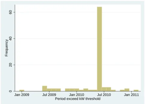
During the period of study, 97 firms are mandated onto the
TOU rate. Figure ?? plots a histogram of the calendar month
in which a firm first crossed the mandatory TOU threshold. The modal month in which firms cross the mandatory TOU threshold is June 2010, the first month in which the mandatory kW threshold was reduced from 200 to 100. On average the lag between when a firm exceeds the TOU threshold and first faces TOU pricing is 2 months. As we will discuss the modal crossing month and the time lag will inform our empirical approach.
Place Figure?? About Here.
The primary data used to estimate the empirical models con-sist of monthly billing data on electricity usage, peak load, ex-penditure and rate class from 1,785 commercial users serviced
between January 1, 2009 and August 2011. Table ?? provides
descriptive results where means are reported by firm type.
Place Table ?? About Here.
Customers are grouped into one of three firm types: ‘manda-tory switchers’ are customers that were mandated onto TOU pricing during the period of study; ‘always-TOU firms’ identify customers that opt into the TOU rate before August 2007 and are on TOU pricing for the duration of our sample; lastly, ‘non-TOU firms’ are customers that pay a flat-rate throughout the period of study. Mandatory TOU firms comprise our treatment group and in our preferred specification a sub-set of non-TOU firms comprise our control group. In constructing our control group we restricted the sample of non-TOU firms to customers reaching at least 75 kilowatts of peak load in any month, since these firms more closely resembled treatment firms in peak load and usage. In some specifications, we expand the control group to include firms that are always on TOU pricing, since these firms are more similar to treatment firms in observables. We discuss our choice of control group in the empirical approach.
Two pieces of information are made apparent in Table ??.
types. Mandatory TOU firms are the largest firms, in terms of peak load, usage and expenditure. The 1,430 firms always on a TOU rate are the second largest group of customers in size, and firms always subject to a flat-rate are the smallest firms. This points to the importance of controlling for fixed unobservables across treatment and control groups.
Second, we can only infer a critical variable, the ratio of peak to off-peak usage for a subset of firms. We can impute peak and off-peak usage for (i) always TOU firms and (ii) mandatory TOU firms in post-treatment months. In contrast, our imputation cannot recover the ratio of peak to off peak usage for firms in our control group or mandatory TOU firms in pre-treatment months. This prevents us from directly evaluating the impact of the mandatory TOU policy on the load shifting.
A second data set, the load profile data, supplements the billing data by providing information on peak and off-peak usage for a random sample of 1,168 commercial users between January
2009 and December 2010.13 We use these data to calculate the
TOU rate class discount: holding the amount and timing (within each day) of usage fixed, the rate class discount is the decrease in customer bills that occurs simply from switching from a flat to TOU rate. In our analysis, we are interested in isolating the change in electricity expenditure attributable to a behavioral re-sponse; this requires us to net out the change in expenditure due to the rate class discount. To calculate this discount, we select the largest 5 percent of flat-rate firms in the load profile data, since these firms are closest to the TOU threshold, and calcu-late the bill counterfactual under TOU prices. The discount is calculated by firm-month, but we average up to an annual
mea-sure.14 Table ?? shows the TOU discount for the top two usage
vigintiles among flat-rate firms. On average, the TOU discount reduces kWh expenditures by 3.5 percent and kW expenditures by 40.7 percent.
Place Table ?? About Here.
13These data are comprised of customers who always face a
time-invariant rate structure or always face a TOU rate structure; we do not observe mandatory switchers in these data.
14Our load profile data extend through December 2010, so we assign the
IV IDENTIFICATION AND EMPIRICAL APPROACH The threshold-based treatment assignment mechanism forms the basis of our empirical approach. We exploit the change in rate structure that occurs at the 100kW threshold to implement a regression discontinuity design, allowing identification to arise from the sharp change in treatment status on either side of the threshold. The forcing variable in our setting is defined as the peak load in June 2010. If firms lack precise control over this variable, then idiosyncratic factors will push some households over the threshold but not others. In our setting, it would be extremely difficult, if not impossible, for a firm to precisely
con-trol peak load.15 One implication of this imprecision is that
within the neighborhood of the threshold, assignment to control and treatment is as good as random. In our sample, all firms breaching the active kW threshold are eventually switched onto TOU pricing.
To isolate the effect of mandatory TOU pricing on usage, peak load and expenditure, we estimate an OLS model using a two-step procedure that controls for potential mean reversion. This implementation of OLS allows us to control for firm-specific trends and seasonality using the full panel of data (December 2009-June 2011), and then estimate treatment effects using data from June 2010, the modal treatment assignment month, on-wards. In the first stage the sample is comprised of the months spanning December 2009-June 2011, which includes six months before crossing and allows us to identify pre-existing trends. We
control for firm-specific trends (ηi) and month-by-year fixed
ef-fects (αt) by estimating,
(1) yit =αt+ηit+it
The dependent variableyit is the natural log of either peak load,
total usage or expenditure by customer i in montht. Residuals
from this regression, denoted by ˜y, are used in the second stage.
We then restrict the sample to post-May 2010 and estimate OLS on a many-differences model,
(2) y˜t−y0˜ =βIit+f(˜yi0) +λit
15Managers would need to know the hour during which peak demand
occurred and then have the ability to control usage during this period. In our setting, firms are informed of peak load and monthly usage in monthly increments. Further, these bills do not report the timing of peak load.
The dependent variable is the change in the natural log of usage,
peak load or expenditure between periodtand June 2010, where
t = 0 corresponds to June 2010. Period t includes the months
spanning August 2010, the modal month when firms first face
TOU pricing, to June 2011. TOU pricing is denoted by I, an
indicator variable set equal to one if firm i is on the mandatory
TOU schedule in June 2010. In the displayed results we allow
f(˜yi0) = ˜yi0.16
The primary motivation for deploying this approach is that it controls for mean reversion. In our setting, some firms with a large transitory shock to their peak load may exceed the assign-ment threshold one period, only to revert to a lower peak load from the likely more moderate shock to follow. Neglecting this feature of the data generating process may significantly bias the estimated treatment effect downwards, and perhaps lead to the incorrect inference that firms respond to the new price regime by conserving energy and reducing their peak load. By including the crossing period level of the dependent variable as a second-stage control, we address this issue.
Our choice of bandwidth is informed by the density of firms around the cutoff and the recognition that as the bandwidth in-creases so does the possibility of heterogeneity in unobservables. Due to the modest number of treated firms in our setting, the density of treated firms around the cutoff is sparse. This moti-vates our decision to use a bandwidth which includes 100 kW above the threshold and 25kW below the threshold. Since the policy was designed to target the largest commercial entities, the sample is sparsely populated above the threshold and much more dense below it.
The density of mass below the threshold raises the possi-bility of avoidance behavior. ‘Bunching’ just below the cutoff would be evident if marginal firms had successfully taken mea-sures to avoid crossing the threshold. Similar to the approach used in Saez [2010] to detect bunching, we generate plots of the distribution of kW and check whether abnormal increases in the
mass appear just below the threshold. Figure ?? compares the
month of June across four years of our sample. Aside from what appears to have been a cool month in June 2009, there are no significant differences in the distribution of peak demand across 16Our results are robust to the inclusion of higher-order polynomials in
˜
yi0. They are also robust to allowing ˜yi0to vary with each difference length
years, and thus no evidence of avoidance behavior. Figure ?? compares the density of peak load in June 2010 with the adja-cent months (May and July, 2010). Again, we find no evidence of bunching.
Place Figures ?? and ?? About Here.
Our empirical strategy is bolstered if no other policies issued by the DPUC or the utility coincided with the introduction of mandatory TOU pricing and were also differentially assigned or available to customers above and below the 100kW threshold. While the DPUC and utility have historically introduced vari-ous programs targeting energy efficiency, these programs were implemented well before 2010, on a voluntary basis, and were available irrespective of proximity to the forcing variable of in-terest to this study.
There is one final potential issue that may be relevant for causal interpretation of the treatment effect estimates, and that is anticipation. If commercial customers invested preemptively in conservation or load-shifting before being switched onto the tariff, the most readily-available channels of behavioral change may have been exhausted. This would attenuate estimates of the treatment effect. Since commercial customers were informed about the mandatory TOU program well before its implemen-tation began, one might view this as an explanation for a null result. However, by not voluntarily switching onto the TOU tar-iff, mandatory switchers have revealed themselves to either a) be unaware of the policy, or b) be aware of the policy but not inter-ested in or able to avail themselves of the savings associated with TOU. If either is true, concerns about firms having engaged in meaningful anticipation are mitigated (though, admittedly, not entirely eliminated).
Our empirical results are estimated on a sample consisting of three firm types - mandatory TOU switchers, flat-rate firms, and firms that are always on TOU (during our sample period). The
latter two firm types serve as potential control groups.17
Re-stricting our control group to include only flat-rate firms allows us to generate internally consistent estimates of the treatment 17Recall that the always-TOU firm type consists of users who
voluntar-ily opted into TOU pricing prior to the introduction of mandatory TOU pricing. Some firms also volunteered onto TOU during the period of our sample, but these are dropped from our dataset.
effect. A hypothetical re-randomization of assignment to control and treatment in this sample would produce consistent estimates as long as unobservables vary smoothly across the threshold. In robustness checks, we expand the set of control firms to include firms that are always on TOU pricing.
V RESULTS
Given that the TOU treatment is comprised of three concurrent price changes - an increase in peak rates, a decrease in off-peak rates and a decrease in the peak load charge - there are multiple margins along which firms may respond to the regime change. In a frictionless world, firms should shift usage from the more expensive peak hours to the less expensive off-peak hours. Given the decrease in the peak load charge, the incentive is also to in-crease peak load. Monthly usage and expenditure could either increase or decrease depending on the firm’s initial load profile and the nature of its response to treatment. With these hy-potheses in mind we turn to a discussion of the results. We first present results on usage, peak demand and expenditure (out-comes that we observe in the data), and then use these results to infer the potential for load shifting.
Results from the estimation of equation ?? are presented
in Table ??. As shown in columns 1 and 2, the switch to the
TOU rate structure does not induce an economically or statisti-cally significant change in usage (kWh) or peak demand (kW). The coefficient estimates reflect an average treatment effect on monthly usage and peak load of -0.7 percentage points and -0.4 percentage points, respectively. With 95 percent confidence, we can rule out effects greater than 1.7 and 1.2 percentage points in magnitude, respectively. Columns 3 and 4 show the treat-ment effect on billed amount and adjusted bill. The difference between these coefficient estimates reflects the fact that prices are lower on the TOU rate. Recall that ‘adjusted’ bill is the observed bill net the rate class discount described in the Data section. After accounting for that structural feature of the pol-icy, mandatory TOU does not change electricity expenditure in a significant way. The point estimate on adjusted bill implies de-creased expenditure of 0.6 percentage points, and the 95 percent confidence interval excludes decreases larger than 1.6 percentage points.
Peak Load. While economic theory predicts that, all else equal, peak load should increase in response to the price change, given the empirical setting it is unsurprising that it does not. It is quite difficult, if not impossible, for firms to predict the hour of peak load. A manager would require knowledge about when peak load can be expected to occur, as well as the gradient of peak load and when each instance in the rank order occurs. This is an exceedingly complicated task due to the high degree of het-erogeneity between firms and across months within a firm. The difficulty is compounded by the fact that firms receive electricity bills in monthly increments and that the bill does not even re-port the time of the peak occurrence. One approach a manager might take is to hypothesize that the firm’s peak would occur concurrently with the system peak. However, the data reveal that only 2.7 percent of peak load instances occur during the system peak, and a mere 14.0 percent occur on the same day. Further, within a firm, the timing of the peak load instance changes over time: only 28.9 percent occur during the firm’s modal peak hour-of-day.
Another possible explanation for the lack of a kW response is that many firms face competing price incentives during the peakiest hour of the month: the peak load charge is lower but the on-peak usage charge is higher. In contrast, for firms whose
peak load occurs duringoff-peak hours, there is an unambiguous
incentive to increase peak load during off-peak hours. We hy-pothesize that bars and restaurants are the likeliest identifiable segment in our billing sample to have an off-peak non-coincident peak hour (i.e. the highest demand hour in a month to occur during off-peak times). A large fraction (12 percent) of treated firms in our billing data sample fall into this category, accord-ing to the NAICS classifications. A positive treatment effect on kW for these firms would be consistent with the hypothe-sis that firms respond to the financial incentives from TOU. To
test this, we estimate equation ?? including a term that
inter-acts an indicator for the food and beverage NAICS code and the treatment indicator. For the kW regression, the coefficient on the incremental food/beverage effect has a negative sign but it is essentially a tight zero. This result provides evidence of no behavioral response with respect to peak load when there is a unambiguous incentive to increase it. These sector-specific results should be interpreted with caution. Food and beverage establishments may simply be more constrained in terms of their ability to shift load across hours of the day, so the zero result
here is not dispositive.
Load Shifting. The relative increase in price of peak usage
relative to off-peak usage provides a financial incentive to move usage from peak hours to off-peak hours (i.e. ‘load shifting’). We cannot directly observe or test for load shifting since our data do not include the required temporal decomposition. However, one can derive insights about its magnitude from restrictions imposed by the treatment effects on usage, peak demand and
adjusted expenditure (Table??). Given that there are minimal
changes in peak load and total usage, if load shifting were occur-ring then we would expect to observe a decrease in expenditure. We do not. In combination, these statistics impose significant restrictions on the feasible amount of intertemporal usage ad-justments by treated firms.
To gain a sense for the amount of load shifting that is pos-sible while remaining consistent with the estimated treatment
effects, we display in Table ?? the change in monthly bill that
is associated with a hypothesized shift of 0.5-5.0 percent of to-tal usage from peak to off-peak hours. The average reduction in adjusted bill is 0.006, which can be achieved by shifting just over 1.0 percent of usage from peak to off-peak hours. With 95 percent confidence, we can rule out load shifting of greater than 3.0 percent (which results in a 1.6 percentage point decrease in the bill). It is simply impossible to achieve more than very small amounts of load shifting under the constraints imposed by the treatment effect estimates.
Place Table ?? About Here.
Notice that the average firm could save hundreds of dol-lars a year by shifting moderate portions (3-5 percent of us-age) from peak to off-peak, but they do not do so. Nonetheless, the lack of load shifting may be a perfectly rational response by firms. For example, the presence of substantial adjustment costs would rationalize this inaction. Such costs may come in the form of principal-agent obstacles to be overcome within the firm, the presence of costly attention or cognition on the part of the decisions-maker, or potentially a number of other explana-tions. Our results thus suggest that TOU rates must transmit stronger incentives than are present in our setting if they are to achieve the goal of reducing peak load.
V(i) Robustness Checks
To check the robustness of the quantitative results to our choice of control group, we re-estimate the specifications that comprise
Table ??, but this time include the always-TOU customers in
the control group. These firms are the most numerous of the large firms in our dataset (they increase the control group size by 600 percent) and could have been grouped with the flat-rate firms in our primary control group. The always-TOU firms are desirable as controls since they are closer to the treated firms in
their magnitude of electricity usage and load (see Table??). The
results are presented in Table ??, and are economically similar
to the results from our primary specification. However, we now find a statistically significant response in kWh to TOU pricing, though the point estimate remains very small (less than 1 per-cent) and not statistically different from the baseline estimate.
Place Table ?? About Here.
In each of our empirical approaches, we cannot rule out the possibility that a transitory treatment effect is offset by later changes in behavior. One may be concerned that response to treatment may take time if firms are responding by investing in capital. If this hypothesis is correct, then we would expect to see
larger (negative) treatment effects over time. Table ?? presents
estimated treatment effects from equation ?? in three-month
bins according to duration from treatment. Post-treatment data for firms treated in the modal month will appear for 13 months. We find no evidence of the treatment effect increasing as might be expected in a time-to-build capital investment scenario. In fact, in the 10+ month post-treatment bin (which corresponds
to the summer months of 2011) there is a small increase in
usage and expenditure. Of course, this analysis will not capture investments that require more than a one-year time horizon.
Place Table ?? About Here.
Our final robustness check revisits the possibility of avoid-ance behavior via retail choice. In our setting, any firm (in-cluding those mandated onto TOU pricing) has the opportu-nity to choose an alternate supplier for electricity generation. These customers continue to pay transmission and distribution charges to UI, and receive their electricity bill from UI, but the
generation charge is retailer-specific. Public listings of alter-nate suppliers in 2010 and 2011 show that many retailers of-fered time-invariant rates. As such, firms mandated onto TOU could choose to purchase generation at a flat rate from these suppliers. Regulators in Connecticut may have recognized the possibility of this avoidance behavior, since the TOU price in-centive is primarily transmitted through transmission and
dis-tribution charges. Still, as shown in Table ??, a significant
por-tion (approximately one-third) of the peak/off-peak differential is transmitted through the generation charge and is thus avoid-able. When firms on TOU pricing purchase electricity from a flat-rate retail supplier, the overall price differential drops from 8-9.25 cents to 5-6 cents per kWh.
Two pieces of evidence lead us to conclude that firms are not engaging in retail choice-related avoidance behavior. First, there is no change in retail choice patterns on or near June 2010 (the modal crossing month). Second, a simple linear probability model regressing a monthly alternate supplier indicator on a treatment (mandatory TOU) indicator and controls reveals that
treated firms areless likely to switch to an alternate supplier for
generation services. This suggests that firms are not avoiding
mandatory TOU pricing by switching to alternate suppliers.18
V(ii) Bill Changes and Volatility
Much of the resistance to TOU pricing (and dynamic pricing in general) focuses on unexpected bill increases and volatility, both of which may have differential effects across industry type. In this section we create a simple counterfactual against which to analyze the changes in monthly expenditure from TOU pricing. We also calculate the anticipated changes in bill volatility that arise from TOU pricing.
The counterfactual exercise consists of calculating what the TOU customer’s bill would have been if instead the firm had stayed on a flat-rate tariff. During the first month a mandatory firm faces TOU pricing, we calculate the monthly bill if the firm was on a flat-rate (after adjusting for the TOU discount). We
then compare this flat-rate bill to actual expenditure. Table ??
reports statistics on the distribution of bill changes in the first month of TOU pricing by quartile of usage and industry type. In general the observed bill changes are small. On average, bills 18The histogram of retail choice patterns and results from the linear
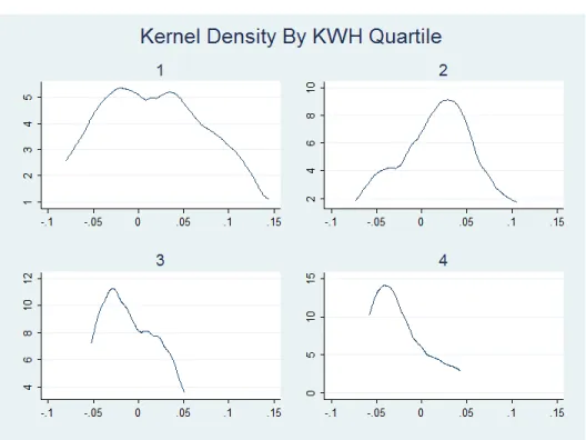
increase by 1.0 percent, and 95 percent of firms experience a bill change of less than 9.4 percent, with many experiencing savings. Larger users in terms of kWh experience savings from TOU pricing while the bottom two quartiles of customers experience a 3.5 percent bill increase. The anticipated bill changes also vary by industry. At the extremes, in the absence of a response, manufacturing users on average incur a 3.9 percent increase in expenditure from this policy, and entertainment/food/beverage firms experience a 3.8 percent decrease in expenditure.
Place Table ?? About Here.
Figures ?? and ?? show k-density plots of the distribution
of bill level changes by kWh quartile and NAICS code, respec-tively. The distribution of effects on the smaller TOU firms has broad support, ranging from nearly a 10 percent savings to a nearly 15 percent bill increase. Recall that while these are the smallest quartile of TOU firms, this group is comprised of rather large electricity users. In this cohort, 95 percent of firms experience bill increases of less than 12.7 percent. The
largest users are much more likely to benefit. Firms in the
top quartile save, on average, 2.7 percent and only 5 percent of these firms experience bill increases exceeding 4.4 percent. Of the NAICS segments, firms in manufacturing, retail, ser-vices/financial and non-profit/religion experience a broad distri-bution of bill changes. By comparison, industrial, educational, entertainment/food/beverage and government sectors are tightly clustered around a zero change in expenditure.
Place Figures ?? and ?? About Here.
While changes in bill levels appear to be small, another crit-icism of TOU pricing is that it will lead to substantial increases in bill volatility. Our setting is well-suited to examine the po-tential of this policy to increase bill volatility. We estimate the coefficient of (unadjusted) bill variation for treated and control firms before and after June 2010. Bill volatility is influenced by seasonality, so we limit our sample of treated firms to those crossing the TOU threshold in the modal month (June 2010). This allows us to compare volatility to an analogous cohort
(con-trol firms), before and after June 2010. Table ?? displays the
means of the coefficients of variation for control and treatment firms before and after June 2010. Bills of treated firms exhibit
an increase in volatility of 10.9 percent (on average). However, we also calculate a 5.7 percent increase in volatility of control firm bills before and after June 2010, suggesting that much of the increase in volatility for treated firms is attributable to fac-tors aside from TOU pricing. Thus, while TOU may lead to higher bill volatility, it is on average a small change.
Place Table ?? About Here.
VI CONCLUSION
In this study we measure the response of commercial and indus-trial customers to mandatory TOU electricity pricing. Despite a significant shift in marginal prices, customers in our setting do not exhibit reductions in peak load, peak usage, or overall usage. The apparent lack of response implies either that these consumers are perfectly price inelastic (in which case we should not be concerned about efficiency loss in the first place), or that the pricing regime that we study is not effective at transmitting meaningful economic incentives to customers.
Three unique features of our empirical setting allow us to contribute meaningfully to the ongoing debate on how and whether to implement TOU pricing. First, we examine a mandatory de-ployment, which is a rare contrast to the more frequent strategy of allowing customers to opt in voluntarily. Second, in our em-pirical setting the rate change is permanent and as a consequence more likely to induce a response where capital investment is re-quired. Earlier experimental studies that find little response to TOU pricing argue that their results may be due to the tem-porary nature of the rate change (Aigner & Hirschberg [1985]). Yet we continue to find little change in usage or peak load in the first full year following mandatory TOU pricing. Third, our study describes the first C&I setting in the U.S. that does not give customers the opportunity to withdraw from TOU pricing. The opt-out feature that is characteristic of other programs will bias the estimated treatment effect towards a response, since firms capable of substituting within-day usage will remain in the study and those with a low substitution elasticity will exit
the program.19 As such, we provide the first credible measure
in several decades of the impact of a mandatory TOU pricing on C&I firms in the U.S..
The presence of voluntary enrollees on the TOU tariff affects the interpretation of our results and lessons for policy. Our em-pirical focus is on the mandatory feature of the deployment, and as such voluntary adopters are eliminated from our analysis. If, in practice, mandatory TOU pricing programs were not intro-duced in tandem with an opt-in feature, one may wonder how this affects the external validity of our results. However, it is unrealistic to imagine a regulatory setting in which a manda-tory TOU program is not bundled with a voluntary enrollment option; thus our setting contains the fundamental features that any deployment of mandatory TOU pricing would.
While the evidence presented here indicates that the marginal effect of mandatory TOU on firm behavior is negligible, our study is silent on the effectiveness of voluntary TOU. Firms that volunteered for TOU pricing are likely to have either a fa-vorable load profile (low on-peak and high off-peak usage) or the ability to shift from peak to off-peak usage at a low cost. If the latter is true, then a voluntary enrollment approach should at least partially achieve the intended goal of the TOU program. However, we do not test this hypothesis, as our dataset does not provide us with a credible counterfactual group against which to compare the behavior of voluntary adopters.
Finally, our results indicate that concerns over mandatory (as compared to voluntary) TOU pricing in the C&I setting have been overstated. It has been argued that firms involun-tarily switched into time-varying pricing would have to either engage in investments to shift their load profile or face an in-crease in electricity expenditure. In our setting, this is not the case. Even after adjusting for the TOU discount, most firms experience a small (if any) increase in bill volatility and no bill change, with less than 5 percent of mandatory TOU customers experiencing a bill increase greater than 8.5 percent in the first month of the rate change. As such, despite the apparent lack of behavioral change induced by the TOU prices, regulators may still view TOU pricing as a way to smooth the path to more timely and granular dynamic pricing (such as RTP) without ex-posing customers to high bill volatility.
REFERENCES
Aigner, D. and Hirschberg, J., 1985, ‘Commercial/Industrial Customer Response to Time-of-use Electricity Prices:
Eco-nomics, 16(3), pp. 341-355.
Aigner, D.; Newman, J. and Tishler, A., 1994, ‘The Response of Small and Medium-size Business Customers to
Time-of-Use (TOU) Electricity Rates in Israel,’Journal of Applied
Econometrics, 9(3), pp. 283-304.
Allcott, H., 2011? ‘Rethinking Real-time Electricity Pricing,’
Resource and Energy Economics, 33(4), pp. 820-842.
Bertrand, M. ; Duflo, E. and Mullainathan, S. 2004, ‘How Much Should We Trust Differences-in-Differences
Esti-mates,’ Quarterly Journal of Economics, 119(1), pp.
249-275.
Borenstein, S., 2013, ‘Effective and Equitable Adoption of
Opt-In Residential Dynamic Electricity Pricing,’ Review
of Industrial Organization, 42(2), pp. 127-160.
Borenstein, S., 2005, ‘Time-Varying Retail Electricity Prices:
Theory and Practice,’ in Griffin and Puller (eds.),
Electric-ity Deregulation: Choices and Challenges Chicago:
Uni-versity of Chicago Press (Chicago, Illinois, U.S.A.)
Borenstein, S. and Holland, S., 2005, ‘On the Efficiency of Competitive Electricity Markets With Time-Invariant
Re-tail Prices,’ Rand Journal of Economics, 36(3), pp.
469-493.
Chay, K.; McEwan, P. and Urquiola, M., 2003, ‘The Cen-tral Role of Noise in Evaluating Interventions that use
Test Scores to Rank Schools,’American Economic Review,
95(3), pp. 1237-1258.
Faruqui, A. and Sergici, S., 2010, ‘Household Response to Dynamic Pricing of Electricity: A Survey of 15
Experi-ments,’Journal of Regulatory Economics, 38, pp. 193-225.
Faruqui, A. and Sergici, S., 2011, ‘Dynamic Pricing of Elec-tricity in the Mid-Atlantic Region: Econometric Results from the Baltimore Gas and Electric Company
Experi-ment,’ Journal of Regulatory Economics, 40, pp. 82-109.
Jessoe, K. and Rapson, D., (forthcoming), ‘Knowledge is (Less) Power: Experimental Evidence from Residential
Energy Use,’ American Economic Review, 104(4), pp.
1417-1438
Saez, E., 2010, ‘Do Taxpayers Bunch at Kink Points?’
Amer-ican Economic Journal: Economic Policy, 2(3), pp.
180-212.
Steiner, P., 1957, ‘Peak Loads and Efficient Pricing,’ The
Williamson, O., 1966, ‘Peak-load Pricing and Optimal
Ca-pacity Under Indivisibility Constraints,’ The American
Economic Review, 56(4), pp. 810-827.
Wolak, F., 2007, ‘Quantifying the Supply-side Benefits from Forward Contracting in Wholesale Electricity Markets,’
T able I: UI Elec tricit y Pric e Sc hedule N on -T O U TO U Bas ic S er vi ce C h ar ge (F ixe d ) 39.19 66.82 P er -k W D eman d C h ar ge 6.12 3.63 P er -k Wh c os ts S um m er W int er S um m er W int er Peak O ff-pe ak Peak O ff-pe ak S ta nda rd S ervi ce G ene ra ti on 0.1 159 0.1360 0.1060 0.1360 0.1060 D el ive ry Cha rge s 0.0074 0.0074 0.0074 D is tri but ion Cha rge s 0.0208 0.0153 0.0153 Com pe ti ti ve T ra ns m is si on A ss es sm ent 0.0152 0.0152 0.0152 Conge st ion Cos ts -0.001 1 -0.0010 -0.0024 0.0000 -0.0022 0.0000 T ra ns m is si on Cha rge s 0.0260 0.0208 0.0650 0.0000 0.0520 0.0000 T otal p er -k Wh c h ar ge 0.1842 0.1791 0.2364 0.1439 0.2237 0.1439 T otal p er -k Wh c h ar ge , n et ge n er ati on 0.0682 0.0632 0.1005 0.0379 0.0877 0.0379
T able II: Summary Statistics M ea n S t.D ev M ea n S t.D ev Mean S t.D ev # fi rm s M anda tory T O U fi rm s 38.7 24.3 131.7 56.1 7,338 4,297 97 A lw ays T O U fi rm s 33.8 32.0 116.7 159.6 6,179 5,953 1,430 N on-T O U fi rm s 12.8 9.0 51.7 25.0 2,647 1,701 258 M anda tory T O U fi rm s pre -t re at m ent 37.3 23.8 126.6 50.4 7,532 4,551 97 M anda tory T O U fi rm s pos t-t re at m ent 38.3 25.0 130.3 59.1 7,007 4,286 97 M ont hl y Cons um pt ion (000s kW h) M ont hl y P ea k L oa d (kW ) Not es : M ea n a nd s ta nda rd de vi at ions of m ont hl y c ons um pt ion, pe ak l oa d a nd e xpe ndi ture a re pre se nt ed for e ac h group of fi rm s. T he se st at is ti cs a re a ls o provi de d for m anda tory T O U fi rm s pre a nd pos t-t re at m ent . Bi ll ($)
Table III: TOU Rate Class Discount (2010)
kWh kW Fixed Fee ($)
20th Vigintile, Flat Rate Firms Only 3.5% 40.7% -$27.63
19th Vigintile, Flat Rate Firms Only 2.7% 40.7% -$27.63
Notes: kWh and kW figures are mean percentage bill reductions from flat rate firms switching to TOU, holding usage and load constant. The fixed fee discount is constant in dollar terms (and negative).
Table IV: Controlling for Mean Reversion: Effect of TOU Pric-ing on kWh, kW, and Bill
Δln(kWh) Δln(kW) Δln(bill) Δln(bill_adj)
TOU Indicator -0.007 -0.004 -0.017*** -0.006
(0.005) (0.004) (0.005) (0.005)
R-Squared 0.48 0.46 0.49 0.49
Observations 3,087 3,086 3,090 3,090
Notes: Results generated from a specification in which dependent variable is the difference in
demeaned, detrended and deseasonalized ln(kwh) or ln(kw) or ln(bill adjusted) with respect to the modal switching month, June 2010. The control group is comprised of large flat rate firms. Standard errors clustered at the firm. * Significant at the 0.10 level, ** Significant at the 0.05 level, *** Significant at the 0.01 level.
Table V: Load Shifting Simulation Results Shifted % Savings
Amount Mean Mean Min Max
0.5% 0.003 6.244 0.159 19.285 (0.001) (3.723) 1.0% 0.005 12.487 0.319 38.570 (0.002) (7.446) 1.5% 0.008 18.731 0.478 57.855 (0.003) (11.169) 2.0% 0.010 24.974 0.638 77.139 (0.004) (14.892) 2.5% 0.013 31.218 0.797 96.424 (0.005) (18.615) 3.0% 0.016 37.462 0.956 115.709 (0.006) (22.338) 3.5% 0.018 43.705 1.116 134.994 (0.007) (26.061) 4.0% 0.021 49.949 1.275 154.279 (0.008) (29.784) 4.5% 0.023 56.192 1.434 173.564 (0.009) (33.507) 5.0% 0.026 62.436 1.594 192.849 (0.010) (37.230)
Notes:These statistics are calculated by supposing a given percentage of usage is shifted from peak to off-peak hours, using delivery-only prices and billed amount. Sample includes all non-TOU and mandatory TOU firms during months where peak load is between 90-110kW (i.e. "close" to the threshold).
T able VI: Robustness Chec ks: Large Flat-Ra te and Alw a ys-TOU Firms as Con trols Δ ln(kW h) Δ ln(kW ) Δ ln(bi ll ) Δ ln(bi ll _a dj ) T O U Indi ca tor -0.009* -0.005 -0.018*** -0.006 (0.005) (0.004) (0.005) (0.005) R-S qua re d 0.48 0.49 0.47 0.48 O bs erva ti ons 18,712 18,698 18,714 18,713 Not es : Re sul ts ge ne ra te d from a re gre ss ion di sc ont inui ty s pe ci fi ca ti on i n w hi ch de pe nde nt va ri abl e i s t he di ffe re nc e i n de m ea ne d, de tre nde d a nd de se as ona li ze d l n(kw h) or l n(kw ) or l n(bi ll adj us te d) w it h re spe ct to t he m oda l s w it chi ng m ont h, J une 2010. T he c ont rol group i s c om pri se d of vol unt ary T O U a nd l ar ge fl at ra te fi rm s. S ta nda rd e rrors c lus te re d a t t he fi rm . * S igni fi ca nt a t the 0.10 l eve l, ** S igni fi ca nt a t t he 0.05 l eve l, *** S igni fi ca nt a t t he 0.01 l eve l.
Table VII: Dynamic Treatment Effect (RD Specification) Mandatory TOU Δln(kWh) Δln(kW) Δln(bill_adj) 1-3mths post-treatment -0.007 -0.011 -0.002 (0.024) -0.024 -0.022 4-6mths post-treatment -0.017 -0.002 -0.020* (0.013) -0.015 -0.012 7-9mths post-treatment -0.03 -0.015 -0.029 (0.028) -0.028 -0.028 10+mths post-treatment 0.039*** 0.018 0.044*** (0.014) -0.012 -0.013 R-Squared 0.485 0.459 0.488 Observations 3,087 3,086 3,090
Notes: Results generated from a regression discontinuity specification in which dependent variable is the difference in demeaned, detrended and deseasonalized ln(kwh) or ln(kw) or ln(bill adjusted) with respect to the modal switching month, June 2010. The control group is comprised of large flat rate firms. Standard errors clustered at the firm. * Significant at the 0.10 level, ** Significant at the 0.05 level, *** Significant at the 0.01 level.
T able VI II: Summ ary Statistics of Bill Changes Mean S td. D evi at ion 5t h pe rc ent il e 95t h pe rc ent il e O ve ra ll 1.02% 4.70% -5.39% 9.35% By kW h Q ua rt il e Q ua rt il e 1 (L ow ) 3.45% 5.75% -6.95% 12.70% Q ua rt il e 2 3.71% 3.34% -1.62% 10.56% Q ua rt il e 3 -0.34% 3.04% -5.23% 5.09% Q ua rt il e 4 (H igh) -2.73% 2.91% -5.75% 4.35% By N A ICS Indus tri al 3.47% 2.82% 1.48% 5.46% M anufa ct uri ng 3.87% 4.33% -3.52% 9.35% Re ta il 2.16% 4.76% -5.38% 10.56% S ervi ce s/ F ina nc ia l 1.89% 3.59% -3.97% 7.61% E duc at iona l 2.58% 4.45% -5.23% 10.01% E nt ert ai nm ent /F ood/ Be ve ra ge -3.76% 1.41% -5.75% -0.60% N on-P rofi t/ Re li gi ous -0.05% 5.98% -6.95% 12.70% G ove rnm ent 1.02% 4.70% -5.39% 9.35% Not es : W e re port the pe rc ent c ha nge in e xpe ndi ture m anda tory T O U fi rm s i nc ur duri ng t he fi rs t m ont h of T O U pri ci ng. W e c al cua te a fi rm 's m ont hl y bi ll if i t ha d be en on a fl at ra te a nd c om pa re thi s t o a ct ua l expe ndi ture . T re at ed fi rm s a re re st ri ct ed t o t hos e a ss igne d t o T O U in J une 2010. S ta ti st ic s a re pre se nt ed by qua rt il e of c ons um pt ion a nd i ndus try t ype .
Table IX: Coefficient of Bill Variation: Treatment vs. Control Firms
Pre-June 2010 Post-June 2010 Change
Non-TOU Firm 0.24 0.25 5.7%
(0.20) (0.18)
TOU Firm 0.17 0.19 10.9%
(0.12) (0.10)
Notes: The coefficient of variation in unadjusted expenditure is reported for TOU and non-TOU firms before and after June 2010.Treated firms restricted to those assigned to TOU in June 2010. Standard deviations in parentheses.
Figure 1: Defining Key T erms: A 1-Da y St ylistic Load Profile Example 24 0 1 2 3 4 5 6 7 8 9 10 11 12 13 14 15 16 17 18 19 20 21 22 23 1 0 H o ur o f Da y kW (L oa d) A B C Ma x k W (" p e a k l o a d ") A +C = "o ff -p e a k us a g e " (k W h) B = " o n -p e a k u s a g e " (k W h )
Figure 2: Histogram Indicating Month Firms Exceed Mandatory TOU Threshold 0 20 40 60 Frequency
Jan 2009 Jul 2009 Jan 2010 Jul 2010 Jan 2011
Figure 3: Kernel Density of kW, June 2008-2011 0 .0 0 5 .0 1 .0 1 5 .0 2 kd e n si ty kw 0 50 100 150 200 kW
Figure 4: Kernel Density of kW, May-July 2010 0 .0 0 5 .0 1 .0 1 5 kd e n si ty kw 0 50 100 150 200 kW
Figure 6: Kernel Density of Behavior-Invariant Bill Changes by Industry
Figure 7: Dynamic Effects in Event Time: Monthly Consump-tion (kWh) -0.15 -0.05 0.05 0.15 0.25 -6 -5 -4 -3 -2 -1 0 1 2 3 4 5 6 Event Month Mean 95% Confidence
Figure 8: Dynamic Effects in Event Time: Peak Load (kW) -0.15 -0.05 0.05 0.15 0.25 -6 -5 -4 -3 -2 -1 0 1 2 3 4 5 6 Event Month Mean 95% Confidence
Figure 9: Dynamic Effects in Event Time: Adjusted Bill -0.15 -0.05 0.05 0.15 0.25 -6 -5 -4 -3 -2 -1 0 1 2 3 4 5 6 Event Month Mean 95% Confidence