I. ADDITIONAL EVALUATION RESULTS A. Environment
The tests have been performed in a virtualized environment with Mininet 1.0.0 [?]. Mininet is tool to create a virtual network running actual kernel, switch and application code. It is an ideal way to test SDN systems, and is quite flexible about the possible topologies (the topology is defined with Python code).
B. Procedure
Here is the general procedure used to create and run the tests.
The first step is to design the topology and write down the constraints. Let’s consider that the file containing the constraints is namedtest42_cstr.txt. Then we have to translate the topology into Mininet’s language. We have to modify the file test_topo.py and add a class extending Mininet’s Topo class. Let’s call this classTest42. In the constructor we write the instructions necessary to describe the desired topology (switches, hosts, collector, edges). This class will be used by Mininet to build the topology.
We also need a mapping between the host identifiers and actual IP and MAC addresses. Information about how to contact the switches’ OpenFlow port is required. This mapping may vary between different scenarios but we use a generic one for the tests. It is written in the filemapping.txt.
The tools we wrote also require the topology and they derive it from the output of Mininet’snetcommand. This means that we have to run Mininet in order to get this output. We usually launch it with the following command:
sudo mn -custom test_topo.py -topo test42 -mac -switch ovsk -controller remote. This tells Mininet to launch a network described by the class mapped by the test42 identifier in test_topo.py, to use OpenVSwitch-based switches, to set the MAC address of the nodes equal to their identifier and to use a remote controller which defaults to localhost. We can then retrieve the output of the net command and write it into a
test42_topo.txtfile.
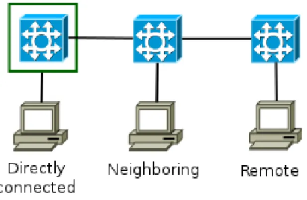
The test network is now running but there is currently no rules defined in the OpenFlow switches. We wrote a script that generates basic routing rules from the mapping and topology files. It can generate the following classes of rules: the broadcast rule, which instructs the switches to forward to all active ports (except the input port) the packets with destination MAC address ff:ff:ff:ff:ff:ff; rules to reach hosts directly connected to the switches; rules to reach hosts connected to direct neighboring switch; and finally rules to reach remote hosts, i.e. hosts with a network distance of at least two hops from a given switch. See Figure 1 for details. When more specific rules are required, they are manually written.
Fig. 1. Three node distance types with respect to the green-squared switch
Once the rules have been inserted in the switches’ flow table, we can start running the test. First we have to run the collector with a proper capture timeout, then run the packets generator. Once the collector has captured the
test packets, it outputs the relevant data in JSON format which can then be given to the constraints checker. The checker then checks each constraint and outputs the results.
C. Binary connectivity
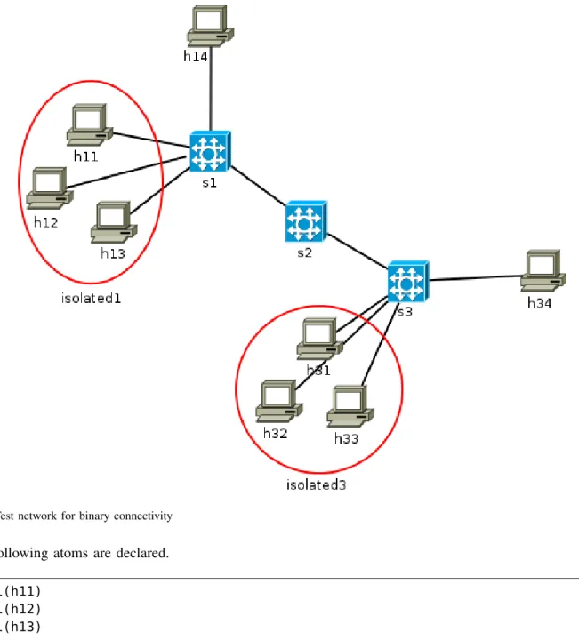
Here we present different tests to check binary connectivity. Let us consider the network shown in Figure 2. We provide the following constraints:
1) Hosts h14 andh34 can reach any other host. 2) Any host can reach h14and h34.
3) Groups isolated1 andisolated3 cannot communicate.
Fig. 2. Test network for binary connectivity The following atoms are declared.
isol1(h11) isol1(h12) isol1(h13) isol3(h31) isol3(h32) isol3(h33)
Specific rules have been defined in order to verify that the binary connectivity constraints is working correctly in different cases: packets from h11to h31are dropped at s1; packets from h12 toh32 are dropped at s2; packets from h13to h33are dropped at s3. This allows us to verify the constraints with empty paths and partial paths.
See Table I for the different test constraints. The fifth column (Checked) refers to the previously enumerated constraints. For each test we provide also the opposite. The first and second tests partially check the first constraint (i.e. hosts h14 and h34 can reach any other host) by checking the traffic between h14 and h34. We expect both constraints to be statisfied.
The third, fourth and fifth tests deal with the empty/partial path issue. Indeed, the 3rd test will not produce any packet for the collector as the injected packets will be immediately dropped at switchs1. The4th test will produce a partial path of length 1, i.e. the path [s1]. The 5th test will produce a partial path of length 2, i.e. [s1 s2].
The last three tests use atom checks and combinations of equality and atom checks. They check the second and third constraints.
Test Constraint Conditions Note Checked Verified 1 allow Hs=h14∧Ht=h34 Equality First
Yes
deny No
2 allow Hs=h34∧Ht=h14 Equality First
Yes
deny No
3 deny Hs=h11∧Ht=h31 Empty path Third
Yes
allow No
4 deny Hs=h12∧Ht=h32 Partial path Third
Yes
allow No
5 deny Hs=h13∧Ht=h33 Partial path Third
Yes
allow No
6 deny isol1(Hs)∧isol3(Ht) Atoms Third
Yes
allow No
7 allow isol1(Hs)∧Ht=h34 Atom, equality Second Yes
deny No
8 allow isol3(Hs)∧Ht=h14 Atom, equality Second Yes
deny No
TABLE I
BINARY CONNECTIVITY TESTS
The implementation is thus working as expected regarding the binary connectivity constraints. See Table II for data on the time spent to perform this test.
Generation 46.97 Injection 30.65 Collection 29.37 Checking 0.357
TABLE II
TIME SPENT BY THE DIFFERENT COMPONENTS. THE TIME IS GIVEN IN MILLISECONDS.
D. Path constraints
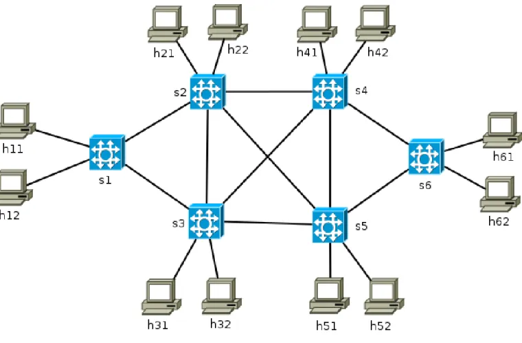
Let us consider the network shown in Figure 4. We define the following constraints. 1) The path from s1 tos4 must go throughs2.
2) The path from s4 tos1 must go throughs3. 3) The path from s1 tos5 must go throughs3. 4) The path from s5 tos1 must go throughs2. 5) The path from s2 tos6 must go throughs4 ors5. 6) The path from s3 tos6 must go throughs4 ors5.
7) All the paths must contain the minimum number of hops.
Fig. 4. Test network for path constraints
The controller is written in the following way. It has the list of path constraints described above. If it receives a packet whose destination is path-constrained, then it attempts to find the shortest path to the required intermediary switch, and retrieve the correct output port. Then it instructs the switch that sent the packet to use this port for all future packets with the same destination MAC by adding an entry to the switch’s flow table. If the controller receives a packet whose destination is not path-constrained, it will simply attempt to find the shortest path to the destination, and modify the switch’s flow table to use the computed path for future packets.
In order to precisely define the paths in the network we have used the -arpargument when launching Mininet. This argument allows the hosts to start with a full ARP table, thus avoiding the need for ARP broadcasts. Indeed, without using a protocol such as STP, all the switches’ ports will remain active and an ARP broadcast will indefinitely loop in the network.
one(h11) one(h12) two(h21) two(h22) three(h31) three(h32) four(h41) four(h42) five(h51) five(h52) six(h61) six(h62)
Fig. 5. Atoms for path constraints test network
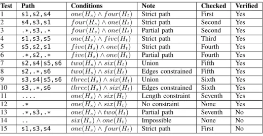
See Table III for a summary of the tests. They consist in verifying each constraint by setting different kinds of paths: strict paths (fully defined for each hop), partial paths (by using the Kleene operator), multiple paths (with the union operator) and length constraints (with the dot symbol).
Test Path Conditions Note Checked Verified
1 s1,s2,s4 one(Hs)∧f our(Ht) Strict path First Yes 2 s4,s3,s1 f our(Hs)∧one(Ht) Strict path Second Yes 3 .*,s3,.* f our(Hs)∧one(Ht) Partial path Second Yes 4 s1,s3,s5 one(Hs)∧f ive(Ht) Strict path Third Yes 5 s5,s2,s1 f ive(Hs)∧one(Ht) Strict path Fourth Yes 6 .*,s2,.* f ive(Hs)∧one(Ht) Partial path Fourth Yes 7 s2,s4|s5,s6 two(Hs)∧six(Ht) Union Fifth Yes 8 s2,.*,s6 two(Hs)∧six(Ht) Edges constrained Fifth Yes 9 s3,s4|s5,s6 three(Hs)∧six(Ht) Union Sixth Yes 10 s3,.*,s6 three(Hs)∧six(Ht) Edges constrained Sixth Yes
11 .... one(Hs)∧six(Ht) Length constraint Seventh Yes
12 .* one(Hs)∧six(Ht) No constraint None Yes
13 .*,s3,.* one(Hs)∧two(Ht) Partial path Seventh No
14 .. six(Hs)∧one(Ht) Impossible None No
15 s1,s3,s4 one(Hs)∧f our(Ht) Strict path First No TABLE III
PATH CONSTRAINTS TESTS
The implementation is behaving as expected. See Table IV for data on the time spent when performing this test.
Generation 69.27 Injection 53.37 Collection 38.72 Checking 4.73
TABLE IV
TIME SPENT BY EACH COMPONENT FOR THE PATH CONSTRAINTS TEST. THE TIME IS GIVEN IN MILLISECONDS
E. Load balancing
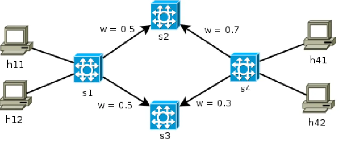
Let us consider the network shown in Figure 6. We define the following constraints. 1) The path from s1 tos4 must be equally load balanced between s2and s3.
Fig. 6. Test network for load balancing
The lack of support of multipath rules in the v1.0.0 of the OpenFlow protocol has forced us to make some modifications to the test procedure for this case: At switchs1, the packets whose destination is directly connected to s4 are sent to the controller, and conversely for the switch s4. The controller handles the load balancing in a flow-based manner. The controller randomly assigns an output port to each different flow (the random number is of course weighted for each link).
The following atoms are declared.
one(h11) one(h12) four(h41) four(h42)
Fig. 7. Atoms for load balancing test network
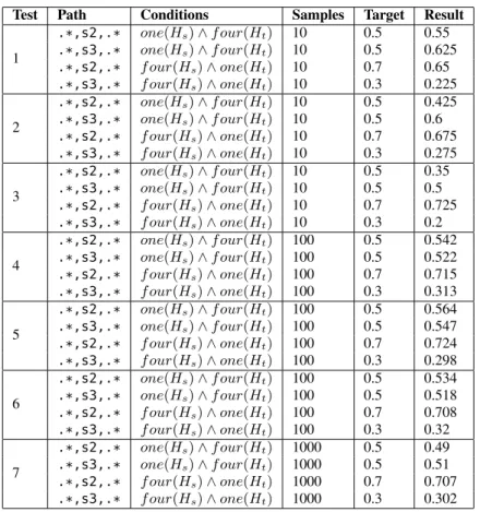
See Table V for a summary of the test. Note that each constraint is tested independently, i.e. the share of traffic going through a given path is not derived from the traffic seen on another path. The first three tests are the same and ran with 10 samples per flow. The next three ran with 100 samples and the last test ran with 1000 samples. These samples were UDP packets whose source port was randomized, ensuring the load balancer would treat them as seperate flows. We can see that as the number of samples increase, the deviation decrease and the values become more precise. The implementation is working as expected, but for future work, we could define an acceptable deviation related to the number of samples and reject the constraint if the result is outside the accepting range.
Test Path Conditions Samples Target Result 1 .*,s2,.* one(Hs)∧f our(Ht) 10 0.5 0.55 .*,s3,.* one(Hs)∧f our(Ht) 10 0.5 0.625 .*,s2,.* f our(Hs)∧one(Ht) 10 0.7 0.65 .*,s3,.* f our(Hs)∧one(Ht) 10 0.3 0.225 2 .*,s2,.* one(Hs)∧f our(Ht) 10 0.5 0.425 .*,s3,.* one(Hs)∧f our(Ht) 10 0.5 0.6 .*,s2,.* f our(Hs)∧one(Ht) 10 0.7 0.675 .*,s3,.* f our(Hs)∧one(Ht) 10 0.3 0.275 3 .*,s2,.* one(Hs)∧f our(Ht) 10 0.5 0.35 .*,s3,.* one(Hs)∧f our(Ht) 10 0.5 0.5 .*,s2,.* f our(Hs)∧one(Ht) 10 0.7 0.725 .*,s3,.* f our(Hs)∧one(Ht) 10 0.3 0.2 4 .*,s2,.* one(Hs)∧f our(Ht) 100 0.5 0.542 .*,s3,.* one(Hs)∧f our(Ht) 100 0.5 0.522 .*,s2,.* f our(Hs)∧one(Ht) 100 0.7 0.715 .*,s3,.* f our(Hs)∧one(Ht) 100 0.3 0.313 5 .*,s2,.* one(Hs)∧f our(Ht) 100 0.5 0.564 .*,s3,.* one(Hs)∧f our(Ht) 100 0.5 0.547 .*,s2,.* f our(Hs)∧one(Ht) 100 0.7 0.724 .*,s3,.* f our(Hs)∧one(Ht) 100 0.3 0.298 6 .*,s2,.* one(Hs)∧f our(Ht) 100 0.5 0.534 .*,s3,.* one(Hs)∧f our(Ht) 100 0.5 0.518 .*,s2,.* f our(Hs)∧one(Ht) 100 0.7 0.708 .*,s3,.* f our(Hs)∧one(Ht) 100 0.3 0.32 7 .*,s2,.* one(Hs)∧f our(Ht) 1000 0.5 0.49 .*,s3,.* one(Hs)∧f our(Ht) 1000 0.5 0.51 .*,s2,.* f our(Hs)∧one(Ht) 1000 0.7 0.707 .*,s3,.* f our(Hs)∧one(Ht) 1000 0.3 0.302 TABLE V LOAD BALANCING TESTS
See Table VI for data on the time spent performing this test.
Samples Total packets Generation Injection Collection Checking 100 3200 1.815 1.686 0.624 0.022 1000 32000 19.169 32.165 6.581 0.186
TABLE VI
TIME SPENT BY EACH COMPONENT WHEN PERFORMING THE LOAD BALANCING TESTS. THE TIME IS GIVEN IN SECONDS.
F. Delay constraints
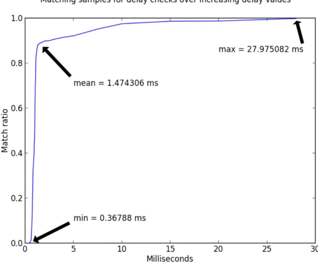
Let us consider the network shown in Figure 8. We would like to define a delay constraint between s1 ands3. The OpenFlow protocol as of v1.0.0 is not able to induce artificial delays. To circumvent this we generated a sample of 1000 test packets and we ran several delay checks on the collected traces. Over the sample, the mean latency is 1.474306 ms with a standard deviation of 2.103613 ms and minimum, maximum latency of resp. 0.367880 ms and 27.975082 ms.
Fig. 8. Test network for delay constraints
See Figure 9 for the details of the measurements. We clearly see that almost 90% of the measurements are under 1.47 ms. Not visible on the graph, we also defined two border checks, one at 0.366 ms and another at 27.976
ms, which is resp. 0.001 ms below and above the minima and maxima. As expected, the first border check gave a matching ratio of 0.0 (all measurements are above the value) and the second one gave a matching ratio of 1.0 (all measurements are under the value). The implementation is thus working correctly.
As for the load balancing constraints, it can be useful to derive a deviation parameter in order to set an accepting range for the delay constraints.