CHAPTER
3
Database Design
Objectives
• To use ER modeling to model data.
• To identify entities and their relationships.
• To describe entities using attributes, multivalued
attributes, derived attributes, and key attributes.
• To know the difference between strong entities and
weak entities.
• To use EER to model inheritance relationships.
• To become familiar with graphical notations in ER and
EER.
• To learn how to translate ER/EER into relation
schemas.
• To understand functional dependencies and use normal
forms to further reduce redundancy. 3.1 Introduction
Before you can store data into the database, you have to define tables. How tables are defined will impact the
database quality. For example, suppose the Department table is defined as shown in Figure 3.1, obviously the table
stores the college information redundantly. Redundancy causes many problems. First, it takes additional space to store redundant data. Second, it slows down the update operation. For example, if the deanId for the Science
college is changed, the DBMS has to exhaustively search for all the records to change the deanId for the Science
college. Third, if the special education department is
too since the information on Education college appears only in one record. The root cause of all these problems is that the two entities Department and College are mixed into one table. This problem can be avoided if the table is derived from a sound database design methodology.
Department Table
deptId name headId collegeId name since deanId CS Computer Science 111221115 SC Science 1-AUG-1930 999001111 MATH Mathematics 111221116 SC Science 1-AUG-1930 999001111 CHEM Chemistry 111225555 SC Science 1-AUG-1930 999001111 SPED Special Education 222223333 EDUC Education 1-AUG-1935 888001111
Figure 3.1
The department and college information are mixed into one table.
A proven sound methodology for database design is the
Entity-Relationship (ER) modeling, which was first proposed by Peter Chen in his 1976 paper “Entity-Relationship Model: Toward a Unified View of Data.” This modeling approach has been widely used for designing logical database schemas. The first step to design a database is to understand the system, know how the system works, and discover what data is needed to support the system, then obtain an ER model and translate the model into the relation schemas, and finally improve the relation schemas using normal forms, as shown in Figure 3.2.
Interact with the user to understand the System ER Modeling Translate the ER model into relation schemas Improve Relation Schemas Using Normal Forms Figure 3.2
An ER diagram can be used to design logical database schemas.
3.2 Entity-Relationship Modeling
An ER model is a high-level description of the data and the
relationships among the data, rather than how data is stored. It focuses on identifying the entities and the relationship among the entities.
An entity is a distinguishable object in the enterprise. An entity has attributes that describe the properties of the entity. For example, a course is an object in the student information system. The course subject, number, name, number of credit hours, and prerequisites are the attributes for the course. All the courses have same type of attributes. A collection of entities of the same attributes is called an
entity set. An entity class (or type) defines an entity set.
An entity class is like a Java class except it does not have
methods. An entity is also known as an entity instance of
its entity class.
3.2.1.1 Key Attributes
Since each entity is distinct, no two entities can have the same values on the attributes. Each entity class has an attribute or a set of attributes that can be used to
uniquely identify the entities. In case there are several keys in the entity class, you can designate one as the
primary key. For example, you can designate the course title
to be the key, assume that every course has a different title.
3.2.1.2 Composite Attributes
A composite attribute is an attribute that is composed of
two or more sub-attributes. For example, the Student entity class has the address attribute that consists of street, city, state, and zipcode.
3.2.1.3 Multivalued Attributes
A multivalued attribute is an attribute that may consist of
a set of values. For example, the Course entity class has the prerequisites attribute. A course may have several prerequisites. Therefore, the prerequisites attribute is a multivalued attribute.
3.2.1.4 Derived Attributes
A derived attribute is an attribute that can be derived or
calculated from the database. A derived attribute should not be stored in the database. For example, you may add an
attribute named numOfPrerequisites to the Course entity class. This attribute can be calculated from the
prerequisites attribute. 3.2.2 ER Diagrams
ER modeling can be described using diagrams. Diagrams make the ER models easy to understand and simple to explain.
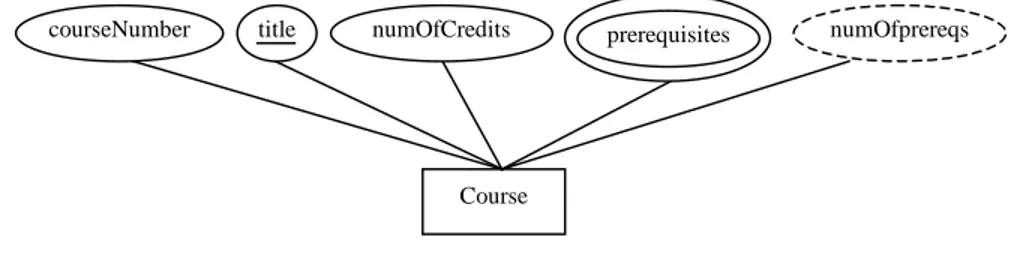
Figure 3.3 shows an ER diagram for the Course entity class and its attributes. An entity class is represented by a
rectangle, an attribute by oval, multivalued attribute by an oval of double borders, and derived attribute by dashed
oval. The primary key attribute(s) are underlined. Figure 3.4 shows an ER diagram for the Student entity class, where address is a composite attribute.
Course
courseNumber title numOfCredits prerequisites numOfprereqs
Figure 3.3
An ER diagram is used to describe the Course entity class and its attributes.
Student
ssn name major address
firstName mi lastName street city state
age
birthDate
Figure 3.4
An ER diagram is used to describe the Student entity class and its attributes.
3.2.2 Relationships and Relationship Classes
An ER model discovers entities and identifies the
relationship among the entities. A relationship between two entities represents some association between them. For
example, a student taking a course represents an enrollment relationship between the student and the course. A
collection of same type of relationships forms a
relationship set. A relationship class (or type) defines a
relationship set. A relationship is also known as a
relationship instance of its relationship class.
in the phrases. For example, the verbs “works” in the phrase “a faculty works in department” implies an employment
relationship between a faculty and a department. The entities are identified from the nouns.
Relationships can have attributes just like the entities. For example, the enrollment relationship may have an
attribute to record when a student is registered for the course.
3.2.2.1 Cardinality Constraints on Relationships
A relationship class establishes the relationships between the entities in the entity classes. An entity in one entity class may be associated with one or more entities in the
other entity class. A cardinality constraint on a
relationship class puts restrictions on the number of
relationships in which an entity may participate. There are four basic types of constraints:
One-to-one: An entity in either entity class may participate
in at most one relationship. For example, a computer user account is assigned to one user and a user can have only one account. So, the relationship between User and Account is one-to-one, as shown in Figure 3.5. The marriage
relationship is one-to-one too.
User Has Account
Figure 3.5
The relationship between User and Account is one-to-one.
One-to-many: An entity in the first entity class may
participate in many relationships, but the entity in the second class may participate in at most one. For example, the relationship between Department and Faculty is one-to-many, because one department may have many faculty and a faculty can be in only one department. Figure 3.6
Department Has Faculty
Figure 3.6
The relationship between Department and Faculty is one-to-many.
Many-to-one: The same as one-to-many, but the entity sets
are reversed.
Many-to-many: An entity in both entity sets may participate
in many relationships. For example, a student can take many courses, and a course can be taken by many students. Figure 3.7 illustrates such constraint.
Student Take Course
Figure 3.7
The relationship between Student and Course is many-to-many.
3.2.2.2 Participation Constraints
The participation constraint specifies whether every entity in an entity class participates in a relationship. If so, it
is called a total participation, otherwise it is called a
partial participation. For example, the participation of
Faculty in the employment relationship with Department is total, because every faculty in the Faculty entity class must work for a department. The participation of Student in the enrollment relationship with Course may be partial,
a semester off.
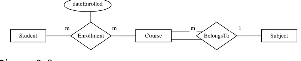
Figure 3.8 shows an ER diagram that describes the relationships among Student, Course and Subject. A relationship class is represented using a diamond. The
constraints on the relationships are denoted using 1 for one
and m for many. A total participation is denoted using
double lines.
Student Enrollment Course BelongsTo Subject
m 1
m m
dateEnrolled
Figure 3.8
An ER diagram is used to describe the relationships. 3.2.2.3 Ternary or n-ary Relationships
The relationships discussed in the preceding sections are binary relationship between two entity classes. It is possible that a relationship may involve three or more entity classes. For example, “a company provides a product for a project” involves three entities Company, Product and Project, as shown in Figure 3.9. A company may provide many products to many projects. A product may be provided by many companies for many projects. A project may use many products from many companies.
Company Product Supply Project m m m name stockSymbol address name color weight name description dateSupplied Figure 3.9
An ER diagram can be used to describe a ternary relationship.
“A company provides a product for a project” is a true ternary relationship, because Company, Product and Project are all associated together and cannot be separated. Some
ternary relationships may be false and should be actually represented using binary relationships. For example, “A student takes a course taught by a faculty” could be erroneously represented using a ternary relationship
involving Student, Course and Faculty. This is wrong because a student and a faculty are not directly associated. The sentence “A student takes a course taught by a faculty” is equivalent to “A student takes a course and a course is taught by a faculty.”
3.2.3 Weak Entities and Identifying Relationship Classes
An entity is called a weak entity if its existence is
dependent on other entities. The other entities are called
owner entities. In contrast, a regular entity is called a
strong entity. For example, a faculty has dependents.
Dependent is a weak entity class that is dependent on its owner entity class Faculty. A relationship between Faculty
and Dependent is called an identifying relationship for the
weak entity. Figure 3.10 shows an ER diagram that describes Faculty and Dependent and their relationship. A weak entity class is represented by a rectangle of double borders and a diamond of double borders represents its identifying
relationship class. Since every weak entity must be
associated with a strong entity, the weak entity class is a total participation of the relationship.
Faculty m 1 has Dependent ssn name birthDate sex Figure 3.10
Dependent is a weak entity that is dependent on Faculty. A weak entity cannot have a key. If an entity has a key, it must be classified as a strong entity set. Suppose Dependent has the attributes ssn, name, birthDate, and sex. If each dependent has a SSN, ssn can be used as the key for the Dependent class. In this case, Dependent becomes a strong entity. It is possible that a dependent may not have a SSN. For example, a newborn may not have a SSN. In this case, Dependent does not have a key, because two dependents may have the same value on name, birthDate, and sex. Dependent has no keys and is a weak entity class. Though Dependent does not have a key, each dependent is distinct and can be identified through its identifying relationship with its
owner entities. The key in the Faculty class along with the name attribute in the Dependent class can form a key to
uniquely identify dependents. The name attribute is referred
to as a partial key. In the ER diagram, a partial key is
underlined by a dashed line, as shown in Figure 3.10. 3.2.4 ER Diagram for a Student Information System Now you can use the ER diagram to describe a student information system as shown in Figure 3.11. Figure 3.12 summarizes the graphical notations for ER diagrams. Figure 3.11 describes the strong entity classes Student, Course, Subject, Department, College, and Faculty, and the weak entity classes Transcript and Dependent, and the
relationships among these entities classes. The ER diagram is self-describing and easy to understand. The ER diagram describes a hypothetical student information system and it is not intended to give a complete description of the
system. The book will use this database in the examples.
Student Enrollment Course
Faculty TaughtBy Subject BelongsTo m 1 m m m m Department m 1 OfferedBy College m 1 BelongsTo WorksIn m 1 1 has Account ssn name address lastName mi firstName email phone street city zipcode state courseId title numOfCredits numOfprereqs prerequisites subjectId name startTime grade dateRegistered name deptId name collegeCode dean lastName mi firstName name startTime ssn name rank email phone lastName mi firstName office numOfdependents since Dependent Owns 1 m 1 birthDate username password birthDate sex since courseNumberr Chairs 1 1 salary age deptId
Figure 3.11
A student information system is represented using an ER diagram.
Strong Entity Class
Weak Entity Class
Relationship Class Identifying Relationship Class Total Participation Relationship Partial Participation Relationship Attribute Key Attribute Derived Attribute Multivalued Attribute Composite Attribute Partial Key Attribute Figure 3.12
An ER diagram uses graphical notations to describe entities, attributes, and relationships.
NOTE: The ER model is not unique. There are many ways to design an ER model. For example, you may consider registration as a weak entity set. So the relationship among Student, Registration, and Course can be drawn as shown in Figure 3.13.
Student m 1 ssn name address lastName mi firstName phone street city zipcode state birthDate Course m courseNumber title numOfCredits numOfprereqs prerequisites Registration has 1 has email age deptId Figure 3.13
Student and Course can alternatively be described through the Registration weak entity class.
3.3 Translating ER Models to Relation Schemas
Once an ER model is created, you can translate it into
relation schemas. This section uses the student information system to demonstrate the translation guidelines.
3.3.1 Translating Strong Entity Classes
For each strong entity class in the ER diagram, create a relation schema. Choose the primary key of the entity class as the primary key of the relation. The attributes are
translated in the following sections. 3.3.2 Translating Simple Attributes
For each simple attribute, create a field in the relation. For example, to translate simple attributes ssn, phone, birthdate, and email in the Student entity class, create fields ssn, phone, birthdate and email in the Student table. You may argue that birthdate is a composite attribute
because it consists of day, month and year. However, it is a bad idea to separate them. SQL has a time type (equivalent to Oracle’s date type) that can be used to represent date and time. You can extract day, month and year from a time or date type value.
3.3.3 Translating Composite Attributes
For each composite attribute, create a field for each simple attribute in the composite attribute. For example, to
translate the composite attribute name in the Student entity class, create fields lastName, mi, and firstName in the
Student table. The Student entity class can be translated as follows:
Student(ssn, lastName, mi, firstName, phone, email, birthDate, street, city, state, zipcode)
3.3.4 Translating One-to-Many Relationships
For each one-to-many relationship type between entity
classes S and T, select one whose cardinality is many, say T, as target. Add the primary key attributes of S (whose cardinality is 1) to T as a foreign key. Add the simple and composite attributes of the relationship class into T. For example, WorksIn is a one-to-many relationship between
Department and Faculty. To translate it, add the primary key attributes in the Department table to the Faculty table as a
foreign key. Add the startTime attribute in the WorksIn relationship class to the Faculty table. The Faculty schema is as follows:
Faculty(ssn, lastName, mi, firstName, phone, email, office, rank, deptId, startTime)
You might wonder why it is a good guideline to add the primary key of S and the attributes of the relationship class to T. The answer is that this reduces redundancy. If you add the primary key of T and the attributes of the relationship class to S, there would be more redundancy in S. For example, suppose you add the primary key of Faculty and startTime to Department, a sample Department table is shown in Figure 3.14. In this Department table, for every CS faculty, the CS department information is stored. This is obviously redundant.
deptId name headId collegeId facultySsn startTime CS Computer Science 111221115 SC 111221111 12-OCT-86 CS Computer Science 111221115 SC 111221115 01-JAN-00 CS Computer Science 111221115 SC 111221119 01-JAN-94 MATH Mathematics 111221116 SC 111221110 11-OCT-76 MATH Mathematics 111221116 SC 111221112 13-AUG-76 MATH Mathematics 111221116 SC 111221116 13-AUG-76 MATH Mathematics 111221116 SC 111221112 01-JAN-00 …
…
A Department Table with Redundancy
Figure 3.14
Department information is stored redundantly in the Department table.
3.3.4 Translating One-to-One Relationships
For each one-to-one relationship type between entity classes S and T, select one with less non-participating entities, as
T, as the target. Add the primary key of S to T as a foreign
key and add the simple and composite attributes of the relationship into T. For example, Owns is a one-to-one relationship between Student and Account. Since every
account belongs to a student, you should select Account as the target. Add the primary key of Student to Account as a foreign key and add the since attribute to the Account relation. The Account schema is as follows:
Account(username, password, ssn, since)
So why is it a good guideline to select the entity class with less non-participating entities as the target? To
answer the question, consider selecting Student as the target for translating the Owns relationship. Add the
primary key username of the Account and the attribute since of the Owns relationship to the Student table. Figure 3.15 shows a sample new Student table. Clearly, the new Student table has many null values because not every student owns an account. If you follow the guideline to translate the
relationship, you can avoid having too many null values.
ssn firstName mi lastName username since
444111110 Jacob R Smith jsmith 9-APR-1985 444111111 John K Stevenson null null 444111112 George R Heintz gheintz 1-SEP-1986 444111113 Frank E Jones null null 444111114 Jean K Smith null null 444111115 Josh R Woo null null
… …
A Student Table with Many null values
Figure 3.15
The Student table contains many null values. 3.3.5 Translating Many-to-Many Relationships
For each many-to-many relationship type R between entity classes S and T, create a new relation schema named R. Let S(k) and T(k) denote the primary keys in S and T,
respectively. Add S(k) and T(k) into R and add the simple and composite attributes of the relationship class into R. The combination of S(k) and T(k) is the primary key in R. Both S(k) and T(k) are the foreign keys in R. For example, Enrollment is a many-to-many relationship between Student and Course. Create a new relation named Enrollment whose attributes include the keys from Student and Course and the attributes dateRegistered and grade. The Enrollment schema is as follows:
Enrollment(ssn, courseId, dateRegistered, grade)
3.3.6 Translating n-ary Relationships
For each n-ary relationship for n > 2, create a new relation schema. Add the primary key of each participating entity class into the relation schema as foreign keys. The
combination of all these foreign keys forms the primary key in the new relation. Add all simple and composite attributes of the n-ary relationship class into the new relation. For example, the ternary relationship in Figure 3.9 can be translated into the following schema:
Supply(companyName, productName, projectName, dateSupplied)
3.3.7 Translating Weak Entity Classes
For each weak entity class W, create a new relation schema named W. Add the primary key of its owner entity class into W as a foreign key and add all simple and composite
attributes of W into the relation. The primary key of the relation is the combination of the primary key from its owner relation and the partial key, if any. For example, Dependent is a weak entity class and its owner class is Faculty. So Dependent can be translated as follows:
Dependent(ssn, lastName, mi, firstName, sex, birthDate)
3.3.8 Translating Multivalued Attributes
For each multivalued attribute, create a new relation schema. Let R be the relation schema that represents the entity class or relationship class that contains the
multivalued attribute. Add the multivalued attribute into the schema and add the primary key attributes of R. The combination of all attributes forms the primary key of the new relation. For example, to translate the multivalued attribute prerequisites in Course, create a new relation schema named Prerequisite as follows:
Prerequisite(courseId, prerequisiteCourseId)
3.4 Enhanced Entity-Relationship Modeling
The ER modeling presented in the preceding section is sufficient to model simple data relationships. A large database system may contain many entity classes and an entity may belong to several entity classes or share properties with entities from different classes. These
relationships correspond to class inheritance in the object-oriented programming. To accurately represent these
relationships, an extension of ER modeling, called Enhanced
ER modeling (EER), was introduced.
3.4.1 Representing Inheritance Relationships
Inheritance models the is-a relationship between two entity
classes. “An entity class A is a special case of an entity
class B” establishes an is-a relationship. A is called a
subclass and B is called a superclass. There are two ways to
discover inheritance relationships—specialization and
generalization. Specialization is the process of defining a
set of subclasses for a superclass. Generalization is the
process of recognizing two or more classes have common
a superclass.
For example, a faculty may be part-time or full-time, so you can define two subclasses PartTimeFaculty and
FullTimeFaculty. You could use the ER diagram in Figure 3.16 to represent their relationships.
PartTimeFaculty Is-a Faculty Is-a FullTimeFaculty
Figure 3.16
PartTimeFaculty and FullTimeFaculty are special cases of Faculty.
The problem with the ER diagram in Figure 3.16 is that it does not describe the relationships between PartTimeFaculty and FullTimeFaculty. They are both subclasses of Faculty. A faculty can belong to only one subclass, either full-time or part-time, cannot be both. A more appropriate notation is shown in Figure 3.17, where PartTimeFaculty and
FullTimeFaculty are connected through a circle. The letter d
inside the circle denotes the subclasses are disjoint. A cup sign facing the superclass is used to represent inheritance.
PartTimeFaculty
Faculty
FullTimeFaculty d
ssn name phone
lastName lastName firstName
sickLeaveHours salary
payRate facultyType
Figure 3.17
PartTimeFaculty and FullTimeFaculty are disjoint subclasses of Faculty.
The Faculty superclass may use an attribute facultyType to determine whether a faculty is a part-time faculty or a full-time faculty. Such an attribute is referred as a
defining attribute.
The double-line connecting between Faculty and the circle implies total participation by Faculty. Each faculty must be either part-time or full-time. It is possible for a partial participation to exist in the inheritance relationship, which allows an entity not to belong to any subclasses. For example, an instructor may be neither full-time faculty nor part-time faculty as shown in Figure 3.18.
PartTimeFaculty
Instructor
FullTimeFaculty d
Figure 3.18
PartTimeFaculty and FullTimeFaculty are instructors, but an instructor may be neither part-time faculty nor full-time faculty.
3.4.2 Representing Overlapping Relationships
If the subclasses are not constraint to be disjoint, their sets of entities may overlap. For example, you may consider an honors course and a distance-learning course as
subclasses of Course. An honors course may be a distance-learning course too, so the HonorCourse and
DistanceLearningCourse classes may overlap. To denote
overlapping relationship, put the letter o inside the
circle, as shown in Figure 3.19.
HonorCourse
Course
DistanceLearningCourse o
Figure 3.19
HonorCourse and DistanceLearningCourse are special cases of Course, but they may overlap.
An entity may belong to more than one specialization
hierarchies. For example, if you wish to further classify faculty by their ranks and by their administrative
functions, you could define AssistantProf, AssociateProf, and FullProf, and DepartmentChair, as shown in Figure 3.20.
PartTimeFaculty Faculty FullTimeFaculty d DepartmentChair AssistantProf d AssociateProf FullProf Figure 3.20
An entity class may have multiple specializations. CAUTION: A common mistake is to over-specialize classes. When defining subclasses, check if a subclass has distinctive attributes that are not shared by other classes. In Figure 3.20,
AssistantProf, AssociateProf, and FullProf don’t have their own distinctive attributes. You could simply add a rank attribute in the Faculty class to describe a faculty’s rank.
3.4.4 Representing Multiple Inheritance
Multiple inheritance means that a subclass may be derived from two or more superclasses. Multiple inheritance can be described in EER. For example, a department chair is both a faculty and an administrator, as shown in Figure 3.21.
Faculty
DepartmentChair
Administrator
Figure 3.21
DepartmentChair is both a faculty and an administrator. 3.4.5 Translating Inheritance Relationships into Relation Schemas
There are three options for translating inheritance relationships to relation schemas.
Option 1: For each superclass P, create a relation schema named P and add all its simple and composite attributes to the schema. For each specialization of P that has a defining attribute, add that attribute to the relation schema. For each subclass of P, create a relation schema, add the
primary key of P into this new relation as a foreign key. In the case, the subclasss has multiple superclasses, declare the primary key of the subclass to be the combination of all the foreign keys. For example, the EER diagram in Figure 3.18 can be translated into the following three relation schemas:
Faculty(ssn, lastName, mi, firstName, phone, facultyType) PartTimeFaculty(ssn, payRate)
FullTimeFaculty(ssn, salary, sickLeaveHours)
Option 2: For each superclass P, create a relation schema named P and add all its simple and composite attributes to the schema. For each specialization of P that has a defining attribute, add that attribute to the relation schema. For each subclass of P, add its simple and composite attributes to P. For example, the EER diagram in Figure 3.18 can be translated into the following relation schema:
Faculty(ssn, lastName, mi, firstName, phone, facultyType, payRate, salary, sickLeaveHours)
The drawback of this option is null values on payRate for full-time faculty and null values on salary and
sickLeaveHours on full-time faculty. The advantage is no join operation is needed to obtain information pertaining to part-time or full-time faculty.
This option is not suitable for multiple inheritance where a subclass has multiple superclasses.
Option 3: For each subclass S, create a relation schema named S. Add all simple and composite attributes of the subclass and its superclass to the schema. The primary key of the new schema is the combination of all keys from the superclasses in case of multiple inheritance. For example, the EER diagram in Figure 3.18 can be translated into the following relation schema:
PartTimeFaculty(ssn, lastName, mi, firstName, phone, payRate) FullTimeFaculty(ssn, lastName, mi, firstName, phone,
salary, sickLeaveHours)
This option is not suitable for overlapping specialization, because it would cause redundancy. For example, if this
option is used to translate the EER in Figure 3.19, a course may be stored in both HonorCourse and DistanceLearningCourse relations.
3.5 Normalization
Figure 3.1 illustrated the redundancy problem in the
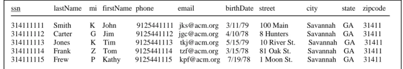
Department table. Using the ER modeling, this problem cannot happen because Department and College are two entity classes and they are translated into two tables. ER modeling can fix many problems like the one demonstrated in Figure 3.1, but redundancy may still exist in the tables translated from the ER diagrams. For example, the Student table shown in Figure 3.22 stores the city and state information redundantly for the same zipcode.
Student Table
ssn lastName mi firstName phone email birthDate street city state zipcode 314111111 Smith K John 9125441111 jks@acm.org 3/11/79 100 Main Savannah GA 31411 314111112 Carter G Jim 9125441112 jgc@acm.org 4/10/78 8 Hunters Savannah GA 31411 314111113 Jones K Tim 9125441113 tkj@acm.org 5/15/79 10 River St. Savannah GA 31411 314111114 Frank Z Tom 9125441114 tzf@acm.org 3/15/78 81 Oak St. Savannah GA 31411 314111115 Frew P Kathy 9125441115 kpf@acm.org 7/19/78 1 Moon St. Savannah GA 31411
Figure 3.22
The Student table stores city and state redundantly for the same zipcode.
This section introduces normalization—a process that
decomposes the relations with redundancy into the smaller relations that satisfy certain properties. These properties
are characterized into normal forms. A relation is said to
be in a normal form if it satisfies the properties defined
by the normal form. Four commonly used normal forms are
introduced in this section: first normal form (1NF), second
normal form (2NF), third normal form (3NF), and Boyce-Codd
normal form (BCNF). Each normal form ensures that a relation
has certain quality characteristics. Normal forms are
defined using functional dependencies. The following section introduces functional dependencies.
3.5.1 Functional Dependencies
The problem in the Student table in Figure 3.22 is that city and state are determined by zipcode. This can be
characterized using function dependencies.
A set of attributes Y is functionally dependent on a set of attributes X if the value of X uniquely determines the value of Y. In other words, for any two tuples in R, if their X values are the same, then their Y values must be same. X is
functionally determines Y. This functional dependency can be described in the following expression:
X Æ Y
So the relationship among city, state, and zipcode is
zipcode Æ city state since for every two tuples with the
same zipcode, their city and state values are the same. NOTE: A functional dependency in a relation must be valid for all the instances of the relation at any time. Once a functional dependency is specified, you need to make sure that the
dependency is not violated at any time. The DBMS can enforce the primary key, foreign key and domain constraints, but it cannot enforce functional constraints. You can write the triggers to enforce functional dependencies. Triggers will be introduced in Appendix G, “Database Triggers.”
3.5.1.1 Inference Rules
Given a set of functional dependencies, you can derive new functional dependencies using the following inference rules:
Reflexivity Rule: If X ⊇ Y, then X Æ Y.
Augmentation Rule: If X Æ Y, then XZ Æ YZ.
Union Rule: If X Æ Y and X Æ Z, then X Æ YZ.
Decomposition Rule: If X Æ YZ, then X Æ Y and X Æ Z.
Transitivity Rule: If X Æ Y and Y Æ Z, then X Æ Z.
Pseudo-transitivity Rule: If X Æ Y and WY Æ Z, then WX Æ
Z.
These rules are intuitive and easy to prove. Here are the examples to prove the reflexivity rule and the
pseudo-transitivity rule. For any two tuples t1 and t2, if t1[X] = t2[X], then t1[Y] = t2[Y] since Y is a subset of X.
Therefore, X Æ Y.
To prove the union rule, consider two tuples t1 and t2 with
t1[X] = t2[X]. Since X Æ Y, t1[Y] = t2[Y]. Since X Æ Z,
t1[Z] = t2[Z]. Therefore, t1[YZ] = t2[YZ].
To prove the pseudo-transitivity rule, consider two tuples
t1 and t2 with t1[X] = t2[X]. Since X Æ Y, WX Æ WY (by the
augmentation rule). Since WX Æ WY and WY Æ Z, WX Æ Z (by
3.5.1.2 Minimum Covers
There are many functional dependencies in a relation. For example, in the Student table in Figure 3.22, you may identify the following functional dependencies:
ssn Æ lastName, mi, firstName
ssn Æ zipCode ssn Æ phone, email ssn Æ birthDate ssn Æ street ssn Æ city, state ssn Æ ssn lastName Æ lastName
Some of the functional dependencies such as ssn Æ ssn and
lastName Æ lastName are trivial and some can be derived
from the others using the inference rules. A functional
dependency X Æ Y is trivial if both sides contain common
attributes.
A minimum cover is a set of functional dependencies F that satisfies the following conditions:
• Every dependency has a single attribute for its
right-hand side.
• For every dependency X Æ A, there is no dependency Y
Æ A for Y ⊂ X.
• No dependency in F can be derived from the other
dependencies in F.
For example, the following is the minimum cover for the Student table. ssn Æ lastName ssn Æ mi ssn Æ firstName ssn Æ phone ssn Æ email ssn Æ zipCode ssn Æ birthDate ssn Æ street zipCode Æ city zipCode Æ state
3.5.1.3 Finding keys Using Functional Dependencies
Typically, database designers first identify a set of
in a relation. Additional functional dependencies can be derived using the inference rules.
You can now define superkey and candidate keys using the
functional dependencies. A superkey is a set of attributes
that determines all attributes in the relation. A candidate
key is a superkey such that no proper subset of it is
another superkey. An attribute is called a key attribute if
it belongs to a candidate key.
A set of attributes, X, may determine many attributes in a
relation. The closure of a set of attributes denoted by X+
is the set of the attributes determined by X. If X is a superkey, then X+ consists of all attributes in the relation.
You can use the inference rules to find all candidate keys in a relation. For example, Let R be a relation schema with
attributes A, B, C, D, E, F, and G and {A Æ CD, B Æ EF, E
Æ G} is a set of functional dependencies in R. To find a
candidate key is to find a minimum set of attributes, K,
such that K Æ R. You only need to consider the attributes
on the left side of the functional dependency expression, because only these attributes can be key attributes. Here is the process of identifying the candidate keys.
Consider attribute A, A Æ ACD.
Consider attribute B, B Æ BEFG.
Consider attribute E, E Æ EG.
Consider combining A and B, AB Æ ABCDEFG. Therefore, AB is
a candidate key.
Consider combining A and E, AE Æ ACDEG.
Consider combining B and E, BE Æ BEFG.
Based on the preceding process, AB is the only candidate key.
3.5.2 First Normal Form (1NF)
A relation is in the first normal form (1NF) if every
attribute value in the relation is atomic. By definition, a relation is already in the 1NF.
3.5.3 Second Normal Form (2NF)
A relation is in the second normal form (2NF) if it is in
1NF and no non-key attribute is partially dependent on any
candidate key. An attribute A is partially dependent on a set of attribute X, if there exists an attribute B in X such
Suppose you mistakenly put the course title as an attribute in the Enrollment relationship, as shown in Figure 3.23. This relationship would be translated as follows:
Enrollment(ssn, courseId, dateRegistered, grade, title)
Student Course m m ssn name address lastName mi firstName email phone street city zipcode state courseId title numOfCredits numOfprereqs prerequisites grade dateRegistered birthDate number Take title Figure 3.23
The title attribute is mistakenly set as an attribute for the Enrollment relationship.
The Enrollment table is not in 2NF, because the candidate key in the table is {ssn, courseId} and title is partially dependent on courseId. To normalize Enrollment into 2NF, you need to remove the non-key attributes that are dependent on the partial key from the relation and place them along with the partial keys in one or more separate tables. The
Enrollment table can be decomposed as follows:
Enrollment(ssn, courseId, dateRegistered, grade) T(courseId, title)
Obviously, T should be combined into Course.
A decomposition is called lossless if no information is lost
in the process. Specifically, assume a relation R is
decomposed into relations R1, R2, ..., and Rk, the
decomposition is lossless if and only if r(R) = r(R1) r(R2)
... r(Rk).
3.5.4 Third Normal Form (3NF)
A relation is in the third normal form (3NF) if it is in 2NF
and no non-key attribute is transitively dependent on any
candidate key. An attribute A is transitively dependent on a
set of attribute X, if there is a set of attributes Z that
Z is called attribute A’s non-key determinant.
For example, the Student relation is not in 3NF, because city and state are transitively dependent on the candidate
key ssn since ssn Æ zipcode and zipcode Æ city state. To
normalize Student into 3NF, you need to remove the non-key attributes that are transitively dependent on the candidate key from the relation and place them along with their
determinants into a new relation. The Student table can be decomposed as follows:
Student(ssn, lastName, mi, firstName, phone, email, birthDate, Street, zipcode)
Zipcode(zipcode, city, state)
3.5.5 Boyce-Codd Normal Form (BCNF)
A relation in 3NF may still face some redundancy problems. For example, suppose the StoreAddress relation has the
attributes street, city, state, zipCode, and store with the
functional dependencies zipCode Æ city, state, and street,
city, state Æ zipCode. StoreAddress is in 3NF because
{store, zipCode, street} and {store, street, city, state} are the candidate keys and every attribute in StoreAddress is a key attribute. As shown in Figure 3.24, city and state information are redundantly stored for the same zipCode. As a consequence, the StoreAddress relation suffers the
insertion, deletion, and update problems.
street city state zipCode store
99 Kingston Street Atlanta GA 31435 Kroger 100 Main Street Savannah GA 31411 Kroger 1200 Abercorn Street Savannah GA 31419 Kroger 100 Main Street Fort Wayne IN 46825 Scott 100 Main Street Savannah GA 31411 Scott 555 Franklin Street Savannah GA 31411 Scott 104 Main Street Atlanta GA 31435 Publix 103 Bay Street Savannah GA 31411 Publix StoreAddress Table
Figure 3.24
StoreAddress is in 3NF, but it still suffers redundancy problems.
BCNF was introduced to tackle this problem. A relation is in
the Boyce-Codd normal form (BCNF) if the determinant of
every non-trivial functional dependency is a candidate key. The StoreAddress relation is not in BCNF, because zipCode is
a determinant in the functional dependency zipCode Æ city,
it into two relations Store(store, street, zipCode) and ZipCode(zipCode, city, state).
NOTE: Normal forms are for measuring the quality of database design. Normalization is a
guideline, not a mandate. Normalization reduces redundancy, but it slows down the performance because you have to perform natural join to obtain information that is now in two or more tables. Suppose your application needs to print student mailing address frequently. If city and state are in the Zipcode table, you have to frequently perform the natural join operations to obtain student name and address from the Student table and the Zipcode table. To improve the performance, you may combine the Zipcode table into the Student table.
NOTE: Normalization has been thoroughly studied in the literature. Many other normal forms were proposed. These forms have theoretical
interests. However, 1NF, 2NF, 3NF, and BCNF are the ones used in practice. There are many
interesting topics that could be covered in a database text. The focus of this book is on practical aspects of the database systems, not to survey normalization theory.
3.5.6 Normalization Examples
Let us now apply the normalization theory in the following examples:
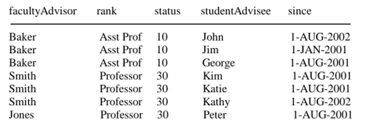
Example 3.1: Suppose relation R consists of the attributes facultyAdvisor, rank, status, studentAdvisee, and since. Figure 3.25 shows an instance of the relation.
facultyAdvisor rank status studentAdvisee since Baker Asst Prof 10 John 1-AUG-2002 Baker Asst Prof 10 Jim 1-JAN-2001 Baker Asst Prof 10 George 1-AUG-2001 Smith Professor 30 Kim 1-AUG-2001 Smith Professor 30 Katie 1-AUG-2001 Smith Professor 30 Kathy 1-AUG-2002 Jones Professor 30 Peter 1-AUG-2001
Figure 3.25
An instance of the relation with attributes faculty, rank, status, studentAdvisee, and since.
The semantic meaning of this relation is as follows:
• Each faculty has a unique rank;
• A faculty’s status is determined by the rank;
• The attribute since records the date when a student is
assigned to a faculty advisor.
You can derive the following functional dependencies from the semantic meaning:
facultyAdvisor Æ rank
rank Æ status
facultyAdvisor, studentAdvisee Æ since
The candidate key is facultyAdvisor and studentAdvisee. Since rank is a non-key attribute that is partially
dependent on the key, this relation is not in 2NF. It can be decomposed into R1(facultyAdvisor, rank, status) and
R2(facultyAdvisor, studentAdvisee, since).
facultyAdvisor is now the key in the relation R1. R1 is not in 3NF, because status (a non-key attribute) is transitively dependent on facultyAdvisor. So, R1 can be further
decomposed into R11(facultyAdvisor, rank) and R12(rank, status).
Example 3.2: Suppose relation R consists of the attributes student, course, teacher, and office. Figure 3.26 shows an instance of the relation.
student course teacher office
Kevin Intro to Java I Baker UH101 Ben Intro to Java I Baker UH101 Kevin Intro to Java I Baker UH101 Chris Intro to Java I Baker UH101 Cathy Intro to Java I Liang SC112 George Intro to Java I Liang SC112 Cindy Intro to Java I Liang SC112 Greg Database Smith SC113
Figure 3.26
An instance of the relation with attributes student, course, teacher, and office.
The semantic meaning of this relation is as follows:
• A student takes a course taught by a teacher;
• A teacher teaches only one course;
You can derive the following functional dependencies from the semantic meaning:
student, course Æ teacher
teacher Æ course
teacher Æ office
The candidate keys are {student, course} and {student, teacher}. Since office (a non-key attribute) is partially dependent on the candidate key {student, teacher}, this relation is not in 2NF. The relation can be decomposed into R1(student, course, teacher) and R2(teacher, office). The functional dependencies in R1 are
student, course Æ teacher
teacher Æ course
R1 is not in BCNF because teacher is a determinant, but it is not a candidate key. Should R1 be further decomposed? It is not a good to decompose it, because the semantic meaning
student, course Æ teacher would be lost if it is
decomposed.
Example 3.3: Suppose a relation R=ABCD has the functional
dependencies AB Æ C and B Æ D. What is the highest normal
form of R? The candidate key in R is AB. Since D is
partially dependent on the candidate key, R is not in 2NF. So, the highest normal for R is 1NF.
Example 3.4: Suppose a relation R=ABCDE has the functional
dependencies A Æ C, B Æ D. What is the highest normal form
of R? The candidate key in R is ABE. Since C is partially dependent on the candidate key, R is not in 2NF. So, the highest normal for R is 1NF.
Example 3.5: Suppose a relation R=ABC has the functional
dependencies A Æ B, B Æ C. What is the highest normal form
of R? The candidate key in R is A. Since C is transitively dependent on the candidate key, R is not in 3NF. So, the highest normal for R is 2NF.
Chapter Summary
This chapter introduced database design. You learned to use the ER diagrams to model database and use the normal forms to improve the database design. The ER diagrams model the database by discovering the entities and analyzing their
relationships. The ER diagrams provide a high-level
description of the database. You learned how to translate ER diagrams into tables. You also learned the functional
dependencies and the normal forms (1NF, 2NF, 3NF, BCNF) and improve the relation schemas through normalization.
Review Questions
3.1 What is an entity, an entity set, and an entity class. 3.2 What are attributes, derived attributes, multivalued attributes, composite attributes, and key attributes? 3.3 What is a relationship, a relationship set, and a relationship class?
3.4 What is cardinality of a relationship? What is a one-to-many relationship, one-to-one relationship, and one-to-many-to-one relationship?
3.5 What is a total relationship? What is a partial relationship?
3.6 What is a weak entity class? What is an identifying relationship?
3.7 What is a ternary relationship?
3.8 Describe the graphical notations for entities, weak entities, relationships, identifying relationships,
attributes, key attributes, derived attributes, composite attributes, and multivalued attributes?
3.9 How do you translate an ER diagram to tables?
3.10 Justify the guidelines for translating one-to-may and one-to-one relationships into tables.
3.11 Give an example of an inheritance relationship. How do you translate an inheritance relationship into tables?
3.12 Give an example of an overlapping relationship. How do you translate an overlapping relationship into tables?
3.13 What is normalization?
3.16 What is a functional dependency?
3.17 What is the first normal form, the second normal form, the third normal form, and BCNF?
Exercises
3.1 Translate the ER diagram in Figure 3.27 into relational schemas. E1 R2 E3 E4 R3 m m 1 m 1 R4 E2 a11 a12 a13 a14 a15 a18 a16 a31 a33 a34 a36 a35 b22 b21 a51 a47 a46 a41 a43 a45 a42 a44 E5 R1 1 m 1 a17 a21 a22 a52 a53 b11 a32 Figure 3.27
You can translate an ER diagram into tables.
3.2 Translate the EER diagram in Figure 3.28 into relational schemas.
E2
E1
E3 d
a11 a12 a13 a14
a21 a22 a23 a24 a31 a32 a33
d1
Figure 3.28
You can translate an EER diagram into tables.
3.3 Design a database for a publishing company. A publishing company has the following entity types: Employee,
Department, Author, Editor, and Book.
Employee has the attributes: ssn (primary key), name (a composite attribute consisting of firstName, mi, and lastName), address (a composite attribute consisting of street, city, state, and zipCode), office, and phone.
Department has the attributes: deptId (primary key), name, and headed. Author has the attributes: ssn (primary key), name (a composite attribute consisting of firstName, mi, and lastName), address (a composite attribute consisting of
street, city, state, and zipCode), and phone. Editor is a subclass of Employee with an attribute specialty that denotes the type of the book (CS, MATH, BUSS, etc.) An
editor may have many specialties. Book has attributes: isbn (primary key), title, and date.
The relationship types are WorksIn, Edits, Writes, Sales, and WorksOn. WorksIn describes the relationship between an employee and a department and it has a time attribute to indicate when the employee started to work for the
department. Edits describes the relationship between an editor and a book. An editor may edit many books and a book is edited by only one editor. Writes describes the
relationship between an author and a book. An author may write several books and a book may be written jointly by several authors. Sales describes the relationship between an employee and a book and it has an attribute to denote the number of the copies sold by an employee. WorksOn describes that an employee works on a book.
Draw the ER diagram for the publishing company database and translate the ER diagram into relational schema.
3.4 Prove the augmentation rule, decomposition rule and union rule.
3.5 Find all candidate keys in the following relations. a. R = ABCDEF AB -> C, C -> DE, F -> E
b. R = ABCDEF A -> D, D -> E, E -> F c. R = ABCDEF AB -> CD, C -> DE, E -> F
3.6 What are the highest normal forms (up to BCNF) of the following relations?
a. R = ABCDEF AB -> C, C -> DE, F -> E b. R = ABCDEF A -> D, D -> E, E -> F c. R = ABCDEF AB -> CD, C -> DE, E -> F