Factors
Affecting Truck
Fuel Economy
V
EHICLE
A
ND
E
NGINE
D
ESIGN
A. Performance Factors
Fuel consumption is a function of power required at the wheels and overall engine-accessories-driveline efficiency.Factors that affect fuel consumption at steady speeds over level terrain are: Power Output-Engine-Accessory-Driveline System
1. Basic engine characteristics; fuel consumption vs. RPM and BHP. 2. Overall transmission and drive axle
gear ratios.
3. Power train loss; frictional losses in overall gear reduction system. 4. Power losses due to fan, alternator,
air-conditioning, power steering, and any other engine-driven accessories. Power Required - Vehicle and Tires
The horsepower required for a vehicle to sustain a given speed is a function of the vehicle’s total drag. The greater the drag, the more horsepower is required. The total vehicle drag can be broken into two main components; aerodynamic drag and tire drag. Factors affecting these components are:
Factors Influencing Drag Aerodynamic – Vehicle speed
Vehicle Frontal area Vehicle Shape
Tire – Vehicle Gross Weight Tire Rolling Resistance Both aerodynamic drag and tire drag are influenced by vehicle speed. It is important, though, to note that speed has a much greater affect on aerodynamic drag than on tire drag, Figure 1.
Gains in fuel economy can be made by either optimizing or reducing some of the factors affecting drag.
B. Type of Vehicle
The type of vehicle affects aerodynamic drag through its size (frontal area) and shape. The following illustration shows two tractor-trailer combinations which, as a result of their shorter height (h2 and h3), have smaller frontal areas than the standard van-type trailer.
Trailer shape has a large impact on the aerodynamic drag of the tractor-trailer combination. Some examples of trailers that have lower aerodynamic drag shapes are: FIGURE 1
Vehicle Speed vs.
Aerodynamic Drag and Tire Drag
Vehicle Speed Drag Force 30 40 50 60 70 80 Tire Drag Aerodynam ic Drag
Where: h1>h2<h3 Frontal Area = FA = (h) x (w) Where: h = Height; w = Width h1
h2
65
Drop frame trailers – Less “Open Air” space under the trailer. This also creates less airflow disturbance in crosswind conditions and thereby reduces the amount of drag.
Sharp Vertical Edge
Rounded Vertical Edge – Maintains “Attached” airflow along the trailer sides, which reduces drag.
Airflow Airflow
Airflow
C. Use of Aerodynamic
Drag Reduction Devices
With van-type trailers, certain add-on devices are capable of reducing a vehicle’s aerodynamic drag. These devices help maintain an “attached” airflow along the trailer sides. Again, an increase in drag occurs when the airflow becomes “detached.”
The favorable impact of roof fairings is maximized when the vehicle is operating in a “head-on” wind condition as shown above. The effectiveness of a roof fairing is reduced when the vehicle encounters a “crosswind” (yaw wind) condition. Also, if the trailer height is lower than the top of the fairing, as in the case of a flat-bed trailer, the fairing increases drag because it increases the vehicle’s frontal area. Use of a “roof shield” is less effective than a “roof fairing” because it doesn’t channel the wind at the sides. Therefore, a “roof fairing” is preferred.
Vertical gap seal devices reduce drag by preventing the airflow from entering the “open air” space between the tractor and trailer. Unlike the roof fairing, the impact of this device is maximized when the vehicle is operating in a yaw wind condition.
D. Engine and Driveline
Characteristics
The use of wide torque band low RPM engines and wide-step top gear transmissions, combined with proper rear axle ratios, leads to fuel economy improvement when operated in the speed and RPM ranges recommended by engine and vehicle manufacturers.
Note that a change in the overall diameter of the drive axle tires can effectively alter the rear axle ratio and could adversely affect fuel economy. The determination whether a drive tire change produces an increase or decrease in fuel economy depends on how much and in which direction engine RPMs are changed.
Side Gap Seal
Vertical Gap Seal Airflow
Also of importance is the amount of gap between the back of the tractor cab and the front of the trailer. The larger the gap, the greater the disruption to the airflow and the resulting drag. This becomes even more important when encountering crosswind conditions (yaw wind). A rule of thumb is for every 10'' over a 30'' gap there is about a 1/10 drop in MPG.
Long Wheelbase Tractor
Yaw Wind Condition Airflow
Gap
67
V
EHICLE
O
PERATION
The effect of tire overall diameter on fuel consumption can be illustrated using an engine fuel map, Figure 2. This is an example of a typical part load brake specific fuel consumption (BSFC) engine map. It shows lines of constant BSFC as a function of engine BHP output (vertical axis) and engine RPM (horizontal axis).
A smaller diameter drive axle tire results in an increase in engine cruise RPMs, from point A to B. At point B the engine is consuming more fuel for the same BHP output.
Proper drive train component matching can provide the most fuel efficient RPM/ ground speed combination to maximize fuel economy. Engine RPMs can be determined using the following formula: Engine RPM=V x TR x AR x (Tire RPM)
60 Where:
V = Vehicle Speed (mph) TR = Transmission Ratio @
Top Gear (e.g. 1.0 for Direct Drive)
AR = Rear Axle Ratio (e.g. 3.70) Tire RPM = Tire Revs Per Mile
(obtained from Goodyear’s Engineering Data Book or www.goodyear.com/truck)
Lines Of Constant BSFC
Increasing Fuel Consumption
Engine Speed - RPM Engine Output - BPH 600 900 1200 1500 1800 1200 360 330 300 270 240 210 180 150 120 90 60 30 A B
A = Cruise Point @ 0% Grade, 80,000 Lbs. GCW
FIGURE 2
A. General
Consider a typical tractor and van combination operating at 80,000 lb. gross combination weight and at 55 MPH on a level highway. No aerodynamic drag reduction devices are used on either the tractor or the trailer. Using bias ply tires in all wheel positions, the approximate distribution of horsepower requirements is as follows:
HP
Item Requirement Percent
Aerodynamic Drag 104 40
Tire Roll Resistance 97 38
Driveline Losses 36 14
Engine Accessories 20 8
257 100
In this example, the horsepower required to overcome bias ply tire rolling resistance is essentially the same as that required to counteract aerodynamic drag. The total horsepower requirement can be lowered with the use of radial ply tires.
Because radial ply tires have lower rolling resistance than bias ply tires, tire horsepower requirements are lower. As a result, fuel economy is improved. And as the proportion of tire horsepower requirement on a vehicle increases, the gain in fuel economy due to using radial truck tires increases. Some examples of tire horsepower requirements as a percentage of total vehicle horsepower requirements are given in Figure 3.
At lower Gross Combination Weights (at the same speed), the horsepower required to overcome the tire rolling resistance is a smaller portion of the total brake horsepower required (BHP). This is also true as speed is increased (at the same GCW). As the vehicle’s aero-dynamics are improved, as in the case of a tractor pulling a tanker trailer rather than a van trailer, the BHP required to overcome aerodynamic drag is reduced. This has the effect of increasing the percent contribution of tire rolling
resistance to the total BHP required. In this case, reducing tire rolling resistance by switching to radials has a greater impact on reducing the total BHP required.
FIGURE 3
Tractor-Trailer Horsepower Requirements By Component
Engine Brake Horsepower Required
400 300 200 100 0 Van Trailer 257 237 179 172 357 334 55 MPH Bias Rad GCW=78,500 Bias Rad GCW=25,000 Bias Rad GCW=78,500 65 MPH Tanker Trailer
Key: HP Required to Overcome –
;;;;;; ;;;;;; ;; ;; ; ; ;;;;;; ;;;;;; ;; ;; ; ; ;;;;; ;;;;; ; ; ;; ;;
Engine Brake Horsepower Required
400 300 200 100 0 55 MPH Bias Rad GCW=78,500 Bias Rad GCW=25,000 Bias Rad GCW=78,500 65 MPH ;;;;;; ;;;;;; Aerodynamic Drag Tire Rolling Resistance Driveline Losses ;; Accessory Losses Accessory Losses ;;;;; ;;;;; ;;;;; ;; ;; ; ; ;;;;;; ;;;;;; ;; ;; ; ; ;;;;; ;;;;; ; ; ;; ;; 38% 211 46% 134 282 260 23% 128 20% 41% 37% 192 42% 34% 17% 15% 32% 28%
Source: Goodyear Maintenance Calculations Source: Mack Truck Engineering, Allentown, PA, Oct. 1992
B. Type of Haul
The ideal type of haul for maximum fuel economy consists of long distance runs at steady moderate speed with a minimum of stop-and-go driving and with a minimum of turning. Shorter runs involve more braking, acceleration and turning. The engine and tires operate at less than optimum conditions. Fuel economy tends to be reduced. In some cases of stop-and-go driving, tires may be operating “cold” part of the time without sufficient continuous driving time for adequate warm-up. A curve of tire rolling resistance vs. warm-up time as obtained from a laboratory test is given in Figure 4.
A 1975 study by the U.S. Department of Transportation and the U.S. Environmental Protection Agencya concluded that the type of haul (local, short-haul, or long-haul trips) has a strong effect on fuel economy improvement attributable to radial tires.
The increased stop-and-go driving of the shorter haul reduces the fuel economy gain due to radials. The results of the study are given below:
Fuel Economy Improvement Due To Radial Tires Versus Driving Mode
Fuel Economy
Driving Mode Improvement
Local 3 to 5%
Short-Haul 4 to 8%
Long-Haul 5 to 9%
aInteragency Study of Post-1980 Goals for Commercial Motor Vehicles; Revised Executive Summary, November 1976. U.S. Department of Transportation and U.S. Environmental Protection Agency.
C. Vehicle Speed
As vehicle speed is increased, horsepower requirements to overcome the aerodynamic drag increase rapidly. There is also an increase in the horsepower required to overcome increasing tire rolling resistance, though this occurs at a lower rate. The sum total horsepower requirement for a tractor-trailer vehicle increases along a curve which has a continually steeper slope as speed is increased. For example, Figure 5shows that the total horsepower requirement at 65 MPH is 40 percent greater than at 55 MPH for the typical tractor and van-type trailer. As a result, fuel economy will fundamentally decrease as operating speed is increased from 55 to 65 MPH.
A calculated curve of the percent difference in MPG versus speed is shown in Figure 6. A reduction in MPG of about eight percent was found for every 5 MPH increase in vehicle speed over 55 MPH. For 65 MPH, this would equal close to a mile-per-gallon loss in fuel economy.
D. Vehicle Gross
Combination Weight
As gross combination weight is increased, tire rolling resistance increases, and vehicle miles per gallon decreases, assuming speed is maintained constant. To verify this point, fuel economy tests were conducted at the Goodyear San Angelo Proving Grounds on Goodyear over-the-road tractor-trailers. Unisteel radial tires were compared to
Super Hi-Miler and Custom Cross Rib bias ply tires on the same vehicles to determine relative miles per gallon.a Figure 7shows the results of the tests along with calculated curves passing through the test points. The effect of vehicle gross combination weight on miles per gallon is shown. Note that as truck gross weight was increased, miles per gallon decreased with both the Unisteel radial tire and the bias ply tire; however, the Unisteel tire gave proportionately greater improvement in fuel economy as truck gross weight was increased.
Tests were run at the San Angelo Proving Groundsato determine the effect of Gross Combination Weight on vehicle miles per gallon, comparing 11R22.5 Unisteel radial to 11-22.5 bias ply tires at 60 MPH. Figure 8shows that at a GCW of FIGURE 6
Vehicle Speed vs.
Percent Change in MPG & BHP
Vehicle Speed (MPH) % Difference in MPG 30 50 40 30 20 10 0 -10 -20 -30 -40 -50 40 50 55 60 70 Vehicle Horse power R equire d Miles-Per-Gallon FIGURE 5 Calculated Horsepower Requirements Tractor, 13.5 Ft. High Van Trailer
vs. Vehicle Speed 11R22.5 Radial Tires GCW=78,500 Lb. Truck Speed–MPH Horsepower Required 20 0 30 100 40 200 50 60 70 300 400 Accessories Driveline Losses Tire Roll. Resist. Aero. Drag
Total Vehicle Requirements
A rule of thumb. Increase of 10 mph = decrease of 1 mpg.
FIGURE 4
Laboratory Tests Truck Tires Rolling Resistance
vs. Warm-Up Time With Capped Air
75 PSI Cold 95 PSI Cold 95 PSI Hot 110 PSI Hot 11-22.5 Bias Ply LR-F, 4760 Lb. Load 11R22.5 Radial LR-G, 5300 Lb. Load Elapsed Time–Minutes
Uncorrected Rolling Resistance–Lb. 0 15
36 30 38 45 40 60 75 90 105 42 44 46 48 50 52 54
Source: Goodyear Maintenance Calculations
69
78,700 lb., the measured MPG advantage of the radial tire was 6.7 percent, while at a GCW of 46,000 lb., the corresponding value dropped to 1.6 percent. This measured reduction in the miles per gallon advantage of radial tires at the lighter load was more severe than theory would indicate. Calculations show that the 6.7 percent advantage should drop to about 3.5 percent at the lighter load.
aThe Effects of Goodyear Unisteel Radial Ply Tires on Fuel Economy. Goodyear Tire & Rubber Company Booklet dated 2/77.
E. Driver
Driver operating procedures are important factors in achieving maximum vehicle fuel economy. The potential benefits of lower vehicle aerodynamic drag, lower tire rolling resistance, and more efficient engines can be offset or even negated by a driver running at a higher speed.
General rules for the driver to follow are:b
• Keep accurate records of fuel used, routes taken and loads carried so
The test data above confirms that the fuel economy advantage of radial truck tires over bial ply tires increases with heavier vehicle Gross Combination Weights.
aTire Parameter Effects of Truck Fuel Economy. R.E. Knight, The Goodyear Tire & Rubber Company. SAE Technical Paper 791043, November 1979.
b“17 Tricks to Save Fuel and Save $$$$”; Pamphlet DOTHS 804 547, June 1979.
you know if you are making any improvements.
• Try progressive shifting, don’t run against the governor on every shift and stay 200-300 RPM below the governor at cruise (See Figure 9). • Stay in as high a gear as possible.
You can’t lug today’s engines if you can maintain speed in any gear. Keep RPM low: below the governor but above the minimum RPM recommended by the engine manufacturer.
• Eliminate unnecessary idling. Shorten warm-up and cool-down times to the minimum recommended by the engine manufacturer. Don’t leave the engine idling while you eat lunch or have coffee.
• Drive defensively.
• Cut down top speed. Each MPH over 55 costs you 2.2% in fuel costs! • Watch the fueling operation. If you
top the tank that valuable liquid could spill or overflow later when you’re parked in the sun.
• Carry as big a load as you can. Run as few empty miles as you can. • Anticipate traffic conditions.
Accelerate and decelerate smoothly.
Tire care can also affect fuel economy. The most important thing a driver can do is to check inflation pressure often with a calibrated tire gauge and make sure that tire pressure is maintained at a recommended high value. (See Figure 14 for effects of inflation pressure on fuel economy.)
FIGURE 7
Miles Per Gallon vs. Truck Gross Weight V=55 MPH Weight Empty Bias Tires Radial Tires San Angelo Tests
12th Gear, G.R.=1.00 Texas Shuttle 10.00R20/10.00-20 Size Tires 13.5 Ft. High Van Cummins NTC 350 Engine Test Points
Gross Combination Weight (Thousands of Pounds)
Miles Per Gallon
20 2.0 3.0 4.0 5.0 6.0 7.0 40 60 80 100 120 140
˚
FIGURE 9 Progressive Shifting Governed RPMMiles Per Hour
0 10 20 30 40 50 60
Idle RPM
Engine RPM
FIGURE 8
Effect of Gross Combination Weight (GCW) on MPG Advantage of Radial Tires
Percent Increase in MPG Radial/Bias Test Data GCW 78,700 46,000 6.7 1.6 6.7* 3.5 Calculated
*Assumed Same Value As Test Data
Source: Tricks to Save Fuel and Save $$$, DOT Pamphlet HS 804547, June, 1978 Source: Goodyear Testing Data
Source: Goodyear CFG Tests and Mathematical Calculations
A. Tire Rolling Resistance
The primary cause of tire rolling resistance is the hysteresis of the tire materials/structure, its internal friction, which occurs as the tire flexes when the vehicle moves. Tire rolling resistance acts in a direction opposite the direction of travel and is a function of both the applied load and the tire’s inflation pressure (See Figure 10).To accurately determine a tire’s rolling resistance, a controlled laboratory test is conducted. One method employed, is to run the tire against an electrically driven 67'' diameter flywheel. A torque cell is used to measure the amount of torque required to maintain a set test speed at a prescribed test load condition. With this torque value, additional adjustments are performed to arrive at the tire’s rolling resistance. The laboratory test provides a procedure where environmental influences (such as ambient temperature, wind, and road surface texture) can be either controlled or eliminated. Also, strict limits are placed on allowable variations in test speed, slip angle, applied load, and specified test inflation. These controls insure test repeatability and allow the accurate assessment of a tire’s true rolling resistance.
Tire rolling resistance is commonly defined in two ways:
a. Pounds resistance per 1000 pounds of load
b. Pounds resistance per pound load (rolling resistance coefficient)
B. Types of Tires
Radial Ply vs. Bias PlyThe significant differences between these two tires are the angle of body plies and the presence of belts. Figure 11shows the basic structural differences. Note that the Unisteel radial tire incorporates a single radial ply and a multiple belt system. The bias ply tire has six to eight diagonally oriented plies and no belt system (although the bias ply tire usually has two fabric “breakers” under the tread with same angle as the plies). One significant advantage of the Unisteel tire is the relatively low internal friction compared to that in a tire using bias ply construction.
The lower internal friction of the Unisteel tire helps minimize operating temperatures and rolling resistance, major causes of tire wear and excess fuel consumption.
Unisteel radial ply tires can provide fuel savings of six percent and more compared to bias ply tires in over-the-road tractor-trailer applications.
Tubeless vs. Tube Type
Laboratory rolling resistance tests indicate that by changing from a 10.00R20 tube type tire to an equivalent 11R22.5 tubeless tire in all wheel positions, a gain of about 2% in miles per gallon can be achieved at 80,000 Ib. GCW. Larger Diameter Tires
Laboratory tests indicate that, under the same load and inflation condition, larger diameter tires produce slightly lower rolling resistance, as in the case of an 11R22.5 versus an 11R24.5. This can produce an improvement in fuel economy coupled with the reduction in engine RPMs due to the larger overall tire diameter on drive axles. (See Section 1-D for the effect of engine RPMs on MPG.)
T
IRE
S
ELECTION
A
ND
M
AINTENANCE
Unisteel Radial Ply Bias Ply
FIGURE 11 Radial Ply vs. Bias Ply Construction
FIGURE 10 Load Direction of Travel Tire Rolling Resistance (Tire Drag)
71
Wide Base Super Single Tires Goodyear Proving Grounds tests show that a fully-loaded tractor-van trailer using Goodyear Super Single Unisteel 15R22.5 tires instead of dual steel radial 11R22.5 tires on tractor drives and on trailer, obtains an average increase of seven to eight percent in MPG.
Commercial fleet testing using loaded tractor-tanker trailers showed a nine percent gain in measured MPG through the use of wide base single 15R22.5 steel
radial tires instead of 11R22.5 steel radial tires in the dual positions. A comparison of the super single versus duals configuration is shown in Figure 12. Retreaded Radial Tires
Goodyear laboratory tests show that the rolling resistance of newly retreaded radial tires is, on the average, the same as radial tires with the full original tread. There are some differences due to type of retread, but all newly retreaded radial tires tested exhibited considerably lower rolling resistance than new bias ply tires. Radial Tires on Trailer Axles
The type of tire used on an axle has a direct impact on the vehicle’s fuel economy. Testing has shown that using radial tires on trailer axles produces over half of the total improvement obtained when converting a vehicle from all bias to all radial. Figure 13details the total percent gain in MPG by switching from bias to radial tires and, of this total gain,
the percentage due to steer, drive, and trailer tires. For maximum fuel economy as well as for best handling, radial tires should be used in all positions of a tractor-trailer unit. Using radial tires especially designed for trailer application will also provide an additional improvement in fuel economy. For example, the radial low profile G114 offers approximately a 10 percent lower rolling resistance than the G159 low profile.
For a vehicle already equipped with radial tires and being switched to another type of radial, the percent contribution by axle to fuel economy will differ from that shown in Figure 13. A rule of thumb for this case is that the front tires contribute about 14 percent of the total, the drive tires about 39 percent, and the trailer tires about 47 percent. It should be noted that the actual percent contribution may differ from the above due to the effects of vehicle loading, tire inflation, and tire type.
FIGURE 13
% Difference in MPG Bias Tires vs. Radial Tires
-Control-All Bias Wide Base Single
Dual Assembly Bias Bias Bias Radial Radial Radial Bias Bias Radial Bias Radial Bias Radial Bias Bias All Radial Radial-Fronts Radial-Trailers Radial-Drives % Gain % of in MPG “All Radial” vs. Control Gain in MPG Radial Fronts 1.0% 17% Radial Drives 1.5% 25% Radial Trailers 3.4% 58% FIGURE 12 Radial Wide Base Single Tire vs. Radial Dual Tire Assembly
% Gain in MPG vs. Control = 5.9%
C. Tire Maintenance
Inflation PressureLaboratory tests were conducted to determine the effect of inflation pressure on the rolling resistance of the 295/75R22.5 G159, G167, and G114 radial truck tires. This laboratory data was used to calculate the corresponding effect of inflation pressure on the fuel consumption of a typical tractor-trailer at 55 MPH on a level highway. The effect of inflation pressure on fuel consumption by axle position was also studied. The results are shown on Figure 14.
A dual tire load of 4250 Ibs./tire and a steer tire load of 5390 Ibs./tire were selected along with a specified inflation pressure of 100 PSI for all tires. Figure 14 shows the percent loss in fuel economy due to the lower inflation pressures.
Operating a loaded tractor-trailer with inflation pressures of all tires as low as 70 PSI results in a calculated reduction in MPG of about five percent. The largest contributor to this loss in MPG is the reduction in inflation pressure of the trailer tires — it alone accounts for half the loss. Varying only the steer tire
inflation pressures results in the smallest percent change in MPG.
It must be noted that the tractor-trailer load affects the percent reduction in MPG due to underinflation. The lighter the GCW, the smaller the percent loss in MPG (for the same reduction in tire inflation).
FIGURE 14
Radial Truck Tire Inflation vs.
Percent Change in MPG
Tire Inflation Varied:
Tire Inflation (psi)
% Difference in MPG GCW =78,780 lbs. V = 55 MPH Front Axle Drive Axles Trailer Axles Front, Drive and Trailer Axles 60 5.0 4.5 4.0 3.5 3.0 2.5 2.0 1.5 1.0 0.5 0.0 -0.5 -1.0 -1.5 -2.0 -2.5 -3.0 -3.5 -4.0 -4.5 -5.0 -5.5 -6.0 65 70 75 80 85 90 95 100 105 110 115 120
A good rule of thumb is that every 10 PSI reduction in overall tire inflation results in about a one percent reduction in MPG.
73
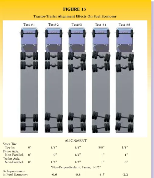
Alignment
For optimum fuel economy on a tractor-trailer, and also for optimum tire wear, tandem drive axles and tandem trailer axles should be maintained in proper alignment. Alignment of the vehicle’s tandem axles should be considered as important as the alignment of the steer axle tires. The importance of this is not only reflected in the loss of MPG due to the increase in tire rolling resistance, but also in the increase in tire wear as a result of the greater amount of side-scuffing. The effects of drive axle and trailer axle alignment is even greater due to the number of tires involved: eight vs. two.
Figure 15illustrates the results of a
Goodyear fuel economy test program run at TRC of Ohio in 1986. These evaluations were Type II tests conducted to SAE J1376 standards. Tests #2 and #3 with steer axle toe-in of 1/4- inch, along with misaligned tandem axles of 1/2-inch total (difference in fore and aft distance between axle center lines, from one side of the vehicle to the other), did not result in a significant loss in MPG versus the specification aligned tractor-trailer. The percent increase in tire rolling resistance due to the slip angles (under .2°) generated by these misalignment conditions is small. What is of greater significance is the loss in tire treadwear life.
Increasing the steer tire toe-in to 3/8-inch and the tandem axle misalignment
to 1-inch in test #4 does produce a loss in MPG which is significant.
The greatest loss in MPG was produced in test #5 where a “dog-tracking” condition was simulated. The trailer tandem axles were misaligned by 1.5-inch though the axles were parallel to one another. The loss in fuel economy was about two percent in addition to increased tread loss.
Treadwear
As the tread is worn down, tire rolling resistance decreases and vehicle fuel economy increases for both radial and bias ply tires. Proving Grounds tests showed about a one percent increase in miles per gallon for radial tires with tread approximately 30 percent worn.a Laboratory tests show about a 10 percent decrease in rolling resistance for both radial and bias ply tires with tread half worn, and a 20 percent decrease for a fully worn tire. (See Figure 16.)
aTire Parameter Effects on Truck Fuel Economy by R. E. Knight, The Goodyear Tire and Rubber Co. SAE Technical Paper No. 791043, November 1979.
FIGURE 15
Tractor-Trailer Alignment Effects On Fuel Economy
FIGURE 16
Effect of Treadwear on Truck Tire Rolling Resistance
Laboratory Data
10.00R20/11R22.5 Sizes At Approx. Rated Dual Load And Inflation, LR-F ‘‘Tips For Truckers’’ FEA/DOT/EPA Document GPO 910-940 Calspan Rep. DOT-TST-78-1 Goodyear Test
Calculation, Based On Goodyear Fuel Economy Test
Bias Ply
Radial ply
Percent Treadwear
Percent Rolling Resistance
0 0 20 20 40 40 60 60 80 80 100 100 ALIGNMENT Steer Tire. Toe-In: 0'' 1/4'' 1/4'' 3/8'' 3/8'' Drive Axle. Non-Parallel: 0'' 0'' 1/2'' 1'' 1'' Trailer Axle. Non-Parallel: 0'' 1/2'' 1/2'' 1'' 0'' *Non-Perpendicular to Frame, 1-1/2'' % Improvement in Fuel Economy: -0.6 -0.8 -1.7 -2.2
Test #1 Test#2 Test#3 Test #4 Test #5
E
NVIRONMENTAL
C
ONDITIONS
A. General
Conditions external to the vehicle can have a strong influence on the fuel economy achieved by a given driver and tractor-trailer/tire combination. Some of the greater influences are exerted by:
Winds Road Surface
Ambient Temperature Terrain
B. Winds
Headwinds and crosswinds reduce truck fuel economy by increasing truck airspeed and/or yaw angle, thus increasing aerodynamic drag. To avoid excessive fuel consumption in sustained strong headwinds, a decrease in truck highway speed is indicated.
Crosswinds also tend to diminish the effectiveness of aerodynamic drag-reducing devices such as cabmounted flow deflectors. Tailwinds are generally beneficial in increasing fuel economy because of the reduced airspeed for a given highway speed. However, if the driver takes advantage of the tailwind and increases his highway speed, the fuel economy gains will be reduced or lost completely.
C. Road Surface
The type of road surface can affect tire rolling resistance. Smooth-textured highway surfaces provide the lowest rolling resistance, while coarse-textured surfaces give the highest tire rolling resist-ance and the lowest fuel economy.
In a test,bit was found that a coarse
chip-and-seal pavement surface gave an increase in passenger tire rolling resistance of 33 percent over that obtained on a typical new concrete highway surface. Relative rankings of the test surfaces were:
Relative Rolling Surface Resistance % Polished Concrete 88 New Concrete 100 Rolled Asphalt (rounded aggregate) 101 Rolled Asphalt (medium
coarse aggregate) 104
Rolled Asphalt
(coarse aggregate) 108 Sealed Coated Asphalt
(very coarse) 133
Another study on passenger tiresc
investigated the effect of road roughness (not surface texture) on rolling losses and concluded:
1. Road roughness increases both rolling and aerodynamic losses (the latter due to vehicle pitching action). 2. Road roughness significantly increases
vehicle rolling losses due to energy dissipation in the tires and suspension. 3. Tests on rough roads led to increases
in rolling losses as large as 20 percent, in addition to introducing increases in aerodynamic drag.
Truck fuel economy may be expected to be influenced in a manner similar to that of passenger cars; by the surface condition of the roadways traveled and by the type of materials used in the pavement—especially in asphalt/ crushed stone mixes. Tire treadwear as well as vehicle fuel economy may be influenced by the particular area of the country being traversed, depending upon the sharpness and hardness of the local crushed stone used in asphaltic concrete road pavement mixes.
bL. W. DeRAAD “THE INFLUENCE OF ROAD SURFACE TEXTURE ON TIRE ROLLING RESISTANCE”, SAE TECHNICAL PAPER 780257 PRESENTED AT THE CONGRESS AND EXPOSITION, COBO HALL, DETROIT, FEBRUARY 27 - MARCH 3, 1978. cSteven A. Velinsky and Robert A. White, “Increased Vehicle Energy Dissipation Due to Changes in Road Roughness with Emphasis on Rolling Losses.” SAE Technical Paper 790653 Presented at Passenger Car Meeting, Dearborn, Michigan, June 11-15, 1979.
75
D. Ambient Temperature
High ambient temperatures reduce tire rolling resistance. High temperatures also reduce atmospheric density, resulting in lower aerodynamic drag. However, fuel economy performance of non-turbocharged diesel engines may be adversely affected by high ambient temperatures, and this would tend to negate some of the gains resulting from lower tire drag and lower aerodynamic drag.Cold weather operation has an opposite effect: tire drag and aerodynamic drag increase at the lower ambient temperatures. The greater thermal efficiency of internal combustion engines at low ambient temperature is usually cancelled by longer warm-up times and longer idling times to maintain cab temperatures during stopover periods. Thus, wintertime fuel economy is generally lower than that obtained in the summer.
E. Terrain
1. GradesMost proving grounds fuel economy testing is done on level terrain, and most simplified calculations relating various truck and tire parameters to truck fuel economy also assume level terrain.
The effect of traveling up a grade is very significant in terms of reducing truck fuel economy. Assuming a one percent grade and an 80,000 pound tractor-trailer, there will be a rearward force exerted by gravity of 80,000 pounds x .01 = 800 pounds.
Proving grounds tests over a measured mile on a road with a 0.1 percent grade consistently showed eight to ten percent lower miles per gallon, comparing going uphill to the west with going downhill to the east. This difference was obtained using a typical tractor-trailer at 55 MPH and at a gross combination weight of 78,500 pounds.
Traveling on a downhill grade improves fuel economy and in hilly country helps to counteract the losses in fuel economy sustained by traveling upgrade.
2. Altitude
As altitude increases, air density and atmospheric pressure decrease. At 5,000 ft. altitude, for example, air density in a standard atmosphere is 14 percent less than at sea level. This percent reduction in air density also applies to reduction in aerodynamic drag, all else being equal.
Tire rolling resistance is not affected by altitude, per se, unless cold inflation pressure is set at lower altitudes and not changed as altitude of operation increases during the course of the trip. For example, a tire with a gauge cold inflation pressure of 100 PSI at sea level, if taken to 5,000 ft. altitude at the same ambient temperature, would have a gauge cold inflation pressure of about 103 PSI. This added inflation would tend to reduce tire rolling resistance.
Altitude effect on engine fuel economy performance depends on the particular engine design and whether or not it is supercharged or tuned for high-altitude operation.
MPG vs. Average Daily Ambient Air Temperature
Average Daily Ambient Air Temperature
MPG 0 20 40 5.4 5.2 5 4.8 4.6 4.4 4.2 60 80 100
*
*
*
*
*
*
*
*
*
*
*
* * **
*
*
*
*
*
*
*
*
*
*
*
** * **
*
*
*
*
*
*
**** *
*
***
T
IRE
D
ESCRIPTION
A
ND
S
PECIFICATIONS
• Static Loaded Radius (SLR)—The distance from the road surface to the horizontal centerline of the wheel, under dual load
• Minimum Dual Spacing—The minimum dimension recommended from rim centerline to rim centerline for optimum performance of a dual wheel
installation
• Loaded Section (LS)—The width of the loaded cross-section
Tire profile or cross-sectional shape is described by aspect ratio (AR): the ratio of section height (SH) to section width (SW) for a specified rim width. For a given tire size, the aspect ratio for a Goodyear radial truck tire is the same as for a bias ply truck tire.
Safety Warning
Serious Injury May Result From: • Tire failure due to underinflation/
overloading/misapplication—follow tire placard instructions in vehicle. Check inflation pressure frequently with accurate gauge.
• Explosion of tire/rim assembly due to improper mounting—only specially trained persons should mount tires. When mounting tire, use safety cage and clip-on extension air hose to inflate.
Cross-Sectional View of Typical Tire
Goodyear Unisteel Low Profile Radial
7. Chafer—A layer of hard rubber that resists rim chafing.
8. Radial Ply—The radial ply, together with the belt plies, withstands the burst loads of the tire under operating pressure. The ply must transmit all load, braking, and steering forces between the wheel and the tire tread.
9. GG Ring—Used as reference for proper seating of bead area on rim.
10. Bead Core—Made of a continuous high-tensile wire wound to form a high-strength unit. The bead core is the major structural element in the plane of tire rotation and maintains the required tire diameter on the rim. Terms Used To Describe Tire/
Rim Combination
• Outside Diameter (OD)—The unloaded diameter of the tire/ rim combination
• Section Width (SW)—The maximum width of the tire section, excluding any lettering or decoration
• Section Height (SH)—The distance from the rim to the maximum height of the tire at the centerline
1. Tread—This rubber provides the interface between the tire structure and the road. Primary purpose is to provide traction and wear.
2. Belts—Steel cord belt plies provide strength to the tire, stabilize the tread, and protect the air chamber from punctures.
3. Stabilizer Ply—A ply laid over the radial ply turnup outside of the bead and under the rubber chafer that reinforces and stabilizes the bead-to-sidewall transition zone.
4. Sidewall—The sidewall rubber must withstand flexure and weathering while providing protection for the ply.
5. Liner—Layers of rubber in tubeless tires especially compounded for resistance to air diffusion. The liner in the tubeless tire replaces the innertube of the tube-type tire.
6. Apexes—Rubber pieces with selected characteristics are used to fill in the bead and lower sidewall area and provide a smooth transition from the stiff bead area to the flexible sidewall. 1 3 5 6 4 8 9 2 7 10 Section Width (SW) Static Loaded Radius (SLR) Flange Height Rim Width Outside Diameter (OD) Section Height (SH) Minimum Dual Spacing Loaded Section (LS)
77
S
UMMARY
The average fuel costs of a given trucking fleet are related to two factors: • Average fleet miles per gallon • Average fuel cost per gallon
While it seems little can be done at the present time to reduce fuel cost per gallon, there are steps that can be taken to increase average fleet miles per gallon.
The miles per gallon achieved by a given truck depends on many factors, the major ones being:
• Vehicle, Engine and Accessory Design and Maintenance
• Vehicle Operation
• Tire Selection and Maintenance • Environmental Conditions
Major fuel-saving steps to apply to trucking operations are:
1. Use fuel-efficient high torque rise, lower RPM engines.
2. Use engine accessories with reduced horsepower requirements, such as clutch fans, synthetic lubricants, etc. 3. Use aerodynamic drag reduction
devices such as flow deflectors and rounded trailer fronts and corners on tractors pulling van-type trailers. Cover open-topped trailers with a tightly-stretched tarpaulin.
4. Use radial tires in all wheel positions, trailer as well as tractor.
5. For best fuel economy, do not allow radial tires to operate below 95 PSI cold inflation pressure.
6. Do not exceed the tire’s rated speed; operate truck fully loaded as much of the time as possible to increase ton-miles per gallon.
APPENDIX
Fuel Economy Test Procedures
There are three fuel economy testprocedures which have been developed by the Society of Automotive Engineers (SAE) and which are currently being used by vehicle manufacturers, tire manufacturers, and by some fleet owners. These offer a standardized method to evaluate either a complete vehicle or a component. Consideration has been given to the effects of environmental conditions (such as those described in Section 4), and their effect on fuel economy results. This is accomplished by requiring the use of a control vehicle which is run simultaneously with the test vehicle. Environmental conditions should affect both vehicles in a similar manner so that for a set of tests, the ratio of either the fuel used or the MPG of the test and control vehicles should be relatively constant even though the actual values of either the fuel used or the MPG may vary from test to test.
A brief description of each procedure is listed along with some of their important requirements.
A. SAE Type I
The SAE Type I procedure is best used to evaluate a component which can be easily switched from one vehicle to another.
The procedure requires two vehicles of the same specification; these are run simultaneously and are identified as vehicles “A” and “B.”
The minimum mileage required for one complete test cycle is 200 miles. This is composed of a 100 mile round trip with the test component on vehicle “B” and then another 100 mile round trip with the test component on vehicle “A.” Since a round trip must start and finish at the same location, the minimum length of the outbound and inbound test leg is 50 miles.
On the outbound test leg vehicle “A” leads vehicle “B” (approximately 200 -250 yard separation). At a point halfway through this test leg (approx. 25 miles) vehicle “A” slows down to allow vehicle “B” to take the lead. At the completion of the outbound leg, fuel tanks are weighed or fuel meter readings are recorded. On the inbound test leg, vehicle “B” leads “A” (same separation distance as outbound leg). Also at a point halfway through the test leg “B” slows down to allow “A” to take the lead. Upon completion, fuel is weighed or meters recorded. The test component is then switched between vehicles and another round trip is made.
The amount of fuel used by vehicles “A” and “B” when they are operating with the test component is compared to that used by both vehicles without the test component.
Test speed — as required
Vehicle loads — within five percent of each other Vehicle
warm-up — representative of fleet operation or not less than 45 minutes at test speed
B. SAE Type II
The SAE Type II procedure is best used to evaluate a component which requires a substantial amount of time for removal and replacement.
This procedure also requires two vehicles, though they do not have to be of the same specification. The vehicles are identified as “C” and “T.” Vehicle “C” is the control vehicle and as such is not modified during the course of the test; vehicle “T” is the test vehicle which is used to evaluate the test component.
The minimum mileage for a complete test is 240 miles. This is composed of three valid test runs of 40 miles (minimum) each with vehicle “T” running a baseline component (control component) and then three valid test runs of 40 miles (minimum) each with vehicle “T” running the test component. Vehicle “T” starts off first; after approximately 5 minutes vehicle “C” begins its run. The test run starts and finishes at the same location.
For each test run the amount of fuel used by vehicle “T” is compared to that used by vehicle “C” in the form of a T/C ratio—the quantity of fuel used by vehicle “T” divided by the quantity of fuel used by vehicle “C.” To be considered valid test runs, three T/C ratios within a two percent band must be obtained. This may require one or more additional test runs. Test speed — as required
Vehicle loads — not required to be the same Vehicle
warm-up — minimum of one hour at test speed Test run time — elapsed time of the
test runs must be within .5%
79
C. SAE Engineering Type
The SAE Engineering Type test provides standardized procedures to evaluate fuel economy for different modes of operation, such as Long Haul Cycle, Short Haul Cycle, Local Cycle, and Transit Cycle. This procedure is more controlled than either the Type I or II tests both in terms of test site conditions and test procedures. The effect of this is reflected in greater repeatability. This procedure is best run on a test track.The procedure requires two vehicles preferably of the same specification. The vehicles are identified as “C” and “T.” Vehicle “C” is the control vehicle and is not modified during the course of the test. Vehicle “T” is the test vehicle which is used to evaluate the test component. Long Haul Cycle:
The minimum mileage for a complete test is 180 miles. This is composed of three valid 30 mile test runs with vehicle “T” running the baseline component (control component) and three valid test runs with “T” running the test component. The start time of the vehicles should be staggered such that they don’t aerodynamically interfere with each other. Halfway through each test run (15 miles) the vehicles are to come to a complete stop, idle for one minute and then accelerate back to the test speed. A test run starts and finishes at the same location. If this procedure is not run on a track it can be handled by running 15 miles outbound and 15 miles inbound.
For each test run a T/C ratio is obtained. This is the MPG of vehicle “T” divided by the MPG of vehicle “C.” A test is considered valid if for the three runs (or more) the spread of T/C ratios doesn’t exceed three percent of the mean value.
Test speed — 55 MPH Vehicle loads — as required Ambient
temperature — 60 to 80°
Wind velocity — average wind speed not to exceed 15 MPH Vehicle
warm-up — minimum of 1 hour at 55 MPH