Simulation and Experimental Validation
of Flow-Current Characteristic of
a Sample Hydraulic Servo Valve
M.S. Sadooghi
1;, R. Sei
1and M. Saadat Foumani
2Abstract. This paper presents a novel model to simulate the ow-current characteristic curve of an electro-hydraulic servo valve in steady state condition. This characteristic curve has three major zones: dead zone, linear zone and saturation zone. By using the presented approach, we can simulate the behavior of all types of valves including under lapped, critical center (zero lapped) and over lapped valves. A hydraulic tester has been designed and constructed for validation of the results. It can test the performance of ow-current and some other properties of the valve. Comparison of experimental and simulated curves describes that the model has an acceptable accuracy in determining the four important valve characteristics: ow gain, saturation ow, saturation current and dead zone. As a result, the model can be used for other studies such as geometrical sensitivity analysis (the ultimate objective of this modeling) or design optimization. Since this model is presented in a computer based algorithm, it can be easily used to observe and measure the eects of change in the parameters of interest (particularly geometrical parameters of the valve) on the ow-current curve.
Keywords: Hydraulic servo valve; Torque motor; Pilot circuit; Spool; Flow-current curve.
INTRODUCTION
Electro-hydraulic systems, as one of the major parts of power production and transmission systems, are widely used in various industries. The main advantages of these systems are high power-to-weight ratio, ability to produce and transmit very high power and inherent self-cooling [1]. Control valves are the main part of control process in these systems. These valves are usually employed in two forms: servo and proportional. The manufacturing precisions distinguish proportional valves from servo valves [2]. Their dierences princi-pally can be revealed in the lapping between spool and ports. If this lapping is more than 3% of port diameter, it is a proportional valve and if it is less than 3% of port diameter, it is a servo valve [3]. Overlapped spool in proportional valves leads to less sensitivity to the oil
1. Department of Mechanical Engineering, School of Engineer-ing, Bu-Ali Sina University, Hamedan, P.O. Box 65175-4161, Iran.
2. School of Mechanical Engineering, Sharif University of Tech-nology, Tehran, P.O. Box 11155-9567, Iran.
*. Corresponding author. E-mail: ms [email protected] Received 17 September 2009; received in revised form 12 June 2010; accepted 14 August 2010
pollutions, but on the other hand causes a dead zone characteristic in the ow gain. Under lapped spool or critical center (zero lapped) in servo valves leads to higher response but may increase the instability (in the vicinity of equilibrium position of spool) due to the increasing ow gain [2]. Servo and proportional valves are modeled for various purposes which can be design optimization, linear and nonlinear controller design and sensitivity analysis.
In the last decades, some researchers have pub-lished some works in the eld of servo valves modeling. These papers usually have been founded on derivation of governing dynamic and uid equations of the valve operation. Linearization of these equations leads to a transfer function between input and output variables. In one of the signicant works, Merritt [4] presented a third-order model. Tawc [1] presented a sixth-order model for the rst stage of a servo valve with a feedback spring by using dynamic and uid analysis and aids from Merritt's works. Transfer function input is the current and the output is the spool position. The valve was assumed in the critical center mode. Mokherejee modeled a servo hydraulic valve with a force motor [5]. He studied the sensitivity of ow-current curves to some geometrical characteristics the
valve in the steady state condition. Kim and Tsao [6] presented a fth-order equation for modeling the rst stage of a servo valve with a feedback spring. Noah [7] presented a linearized model for output ow of the valve. He studied the geometrical eects of the ports for optimization of linear operation of the valves. Also he derived governing dynamic equations of apper in a two stage nozzle-apper valve. Eryilmaz and Wilson [2] derived a nonlinear continuous model with the aid of orice equation for the second stage of the valve for all types of lapping. Amirante et al. [8] calculated the uid forces on the spool of an underlapped hydraulic directional valve by Computational Fluid Dynamics (CFD). Also Del Vescovo and Lippolis [9] used CFD method for determination of uid forces on spool.
In overall, it seems that there is no compre-hensive servo valve model that represents all parts of the valve and can simulate both rst and second stages simultaneously. In this work, a sample servo valve without feedback spring is modeled to obtain a simulation of steady state ow-current behavior of the valve. Because of the eects of the geometrical details in sensitivity analysis, we are interested in these details. At rst, torque motor and pilot circuit (rst stage) of the valve are modeled. Then, the CFD method was used for the modeling of the second stage. Finally, by combination of the rst and second stage models of the valve, ow-current characteristic curve is obtained. This simulated curve has been compared with experi-mental curve obtained from the hydraulic tester. MODELING
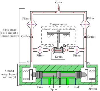
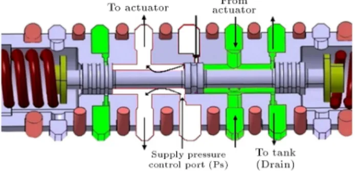
A schematic view of servo valve components is shown in Figure 1. Magnetic solenoid which is actuated by
Figure 1. A schematic view of the valve.
input electrical current inclines the apper towards one of the nozzles. In this situation, the symmetry of pilot circuit is disturbed and the ow rate in the near nozzle becomes less than the far nozzle. It causes a pressure dierence (p) between two sides of the spool. Spool displacement is proportional to this p. Port opening value is a function of the spool displacement. By this mechanism, ports can be controlled electrically with high accuracy. For instance if the spool moves to the left in Figure 1, the high pressure hydraulic uid ows from port \P " to port \B" (load line) via spool body space. Also low pressure hydraulic uid ows from port \A" to storage tank at the same time. In the next sections, simulation of this mechanism by modeling and analysis of the behaviors of all components is presented.
Torque Motor Modeling
Actually, torque motor is a part of the rst stage or amplier stage, but as it is the only electro-mechanical part of the valve, it was modeled separately. The aim of the modeling is derivation of an equation for determination of the applied forces by motor to the armature. An attractive-repulsive torque motor type has been used in this sample valve. A schematic view of the torque motor is depicted in Figure 2. Steady magnetic ux is supplied by four permanent magnets that are made of Alnico5. The control coil was constructed by two parallel coils with 2500 turns. Magnetic ux density of the permanent magnets was measured to be 0.3 T. Electromagnetic model of torque motor circuit is presented in Figure 3. According to this model and using Kirchho rules, we have:
E + Ni = R11+ R44; (1)
E Ni = R33+ R22; (2)
where E, N, i, R and are electrical potential number of turns in the coil, current, reluctance and magnetic ux, respectively. Because of symmetry, we have:
1= 4; (3)
Figure 3. Electromagnetic model of the torque motor.
2= 3; (4)
R1= R4; (5)
R2= R3: (6)
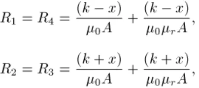
The reluctance R is the summation of air and body reluctances which are the rst and second terms of Equations 7 and 8, respectively [10]:
R1= R4= (k x) 0A +
(k x)
0rA; (7)
R2= R3= (k + x) 0A +
(k + x)
0rA; (8)
where k is the equilibrium distance of armature and body, x is the displacement of the armature end, A is the area normal to the ux path in the air gap, 0 is
the magnetic permeability of air and r is the relative
magnetic permeability of the substance. Flux relations can be derived with the aid of the Equations 1 to 8 as:
1= 2(k x)E + Ni 0A +
2(k x) 0rA
; (9)
2= 2(k+x)E Ni 0A +
2(k+x) 0rA
: (10)
A coecient of 2 appears in the denominators of Equations 9 and 10 because of the existence of two air gaps and two magnetic body sections above and below the armature. So the magnetic ux density is obtained as:
B1= 1=A ! B1=2((E + Ni)0r
rk rx + k x); (11)
B2= 2=A ! B2=2((E Ni)0r
rk + rx + k + x): (12)
To derive an equation for the applied magnetic forces on the armature, at rst, energy in the gap between the armature and the body is calculated. Then by dierentiating the energy equation with respect to the armature displacement (x), an expression is
derived to calculate the force. Equations 13 and 14 represent foregoing energy in attraction and repulsion conditions [10]:
w1=B 2
1(A(k x))
0 ; (Attraction) (13)
w2=B 2
2(A(k + x))
0 : (Repulsion) (14)
The forces are obtained by means of dierentiation:
f1= @w@x1; (15)
f2= @w@x2: (16)
According to Figure 4, these two forces can be seen as a couple that is applied on the armature. The summation of f1 and f2 can be calculated as:
f = f1+ f2
= A2r0[ENik2+kN2i2x+kE2x+ENix2]
(rk + rx + k + x)2(k x)2 : (17)
Armature-Flapper Modeling
Armature-apper set is a medium between the torque motor and the pilot circuit. It transmits the pro-duced torque from motor to the pilot circuit. Main parts of this set are armature, apper and exure tube.
Armature-Flapper Dynamics
Figure 5 shows a free body diagram of the armature and apper assembly. Referring to this gure and using the
Figure 4. A simple model of the apper, armature and exure tube.
Figure 5. Free body diagram of the apper, armature and exure tube.
torque balance, the governing dynamic equation of the armature and apper can be expressed as:
Tt Ts (F1 F2)r = J + c _; (18)
where Ttis the generated torque by the torque motor,
Ts is the resistance torque of the exure tube, F is
the pilot uid force, r is the radius of the apper from the pivot to the pilot uid forces, J is the polar mass moment of inertia of the apper and the armature, c is the damping coecient of the armature and the apper and f is the rotation angle of the apper. Since the
sample valve is studied in steady state condition, the dynamic eects due to the motion of the armature-apper mechanism are not considered in this work. Indeed, in each step, the output ow of the valve or other quantities have been modeled or measured in the state which input current has a constant value. This implies that the right side of Equation 18 equals zero. So it can be said that the steady state equation of the armature-apper is:
Tt Ts (F1 F2)r = 0: (19)
According to Figure 5 and by use of Equation 17, Tt
can be written as: Tt=A
2
r0[iENk2+i2kN2x+kE2x+iENx2]
(rk + rx + k + x)2(k x)2 La(20);
where La is the arm length of the armature. In the
exure tube it can be assumed that Ts= Ksf where
Ks is the stiness of the exure tube. Also r = xff
and La = xf [1] (xf is the apper displacement).
Equation 20 was validated by an experiment. In this test Tt was measured as a function of input current
when f and xf are xed on zero (xf = f = 0) by
applying extra input current to the torque motor. The
armature and the apper are considered as a rigid set. According to Figure 5, if f = 0 then x = xf = 0. This
constraint omits the eects of the exure tube stiness for this specimen. The comparison of experimental and theoretical data (obtained from Equation 20 with x = xf = 0) is shown in Figure 6. As can be seen, the
calculated values from Equation 20 have an acceptable accuracy.
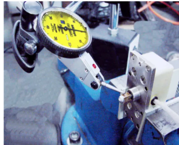
Flexure Tube Stiness
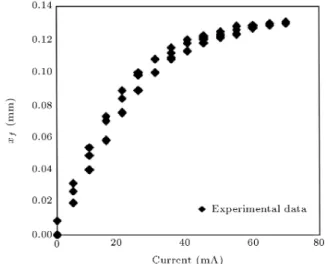
The stiness of the exure tube was obtained by an experimental procedure. As it is shown in Figure 7, the torque motor is separated from the valve set. Displacement of the apper (xf) versus the input
current was measured in the absence of hydraulic uid. In Figure 8 the results of this experiment are shown. After some algebraic calculations, Tt versus f was
obtained and plotted in Figure 9. The slope of the
Figure 6. Comparison of the simulated torque with the experimental torque as functions of the input current when xf = f = 0.
Figure 7. Measuring the apper displacement in terms of the input current (torque motor is separated from the valve set).
Figure 8. Flapper displacement versus input current (in the absence of pilot uid forces).
Figure 9. Stiness of the exure tube.
tted line is the stiness of the exure tube. In this test, this value was found to be 12.86 N.m/rad. FLUID ANALYSIS OF PILOT CIRCUIT Fluid Forces
According to Figure 10, all of the applied forces on the apper due to the hydraulic uid of the pilot circuit can be listed as follow [11]:
- Pressure exerted force (FP) is the major force:
FP =4d2npnKq: (21)
- Momentum exerted force (FM) which is presented
by:
FM = 8(Cd(L + xf))2pnkq: (22)
Figure 10. Fluid forces on the apper.
- Bernoulli force (FB) which is:
FB= (Cddn)2
ln
d
e
dn
1 2
" 1
dn
de
2#)
pnKs: (23)
In these equations kq is obtained from:
kq= 1
1 + 16L +xf
dn
2: (24)
Finally, the resultant force that is applied to the apper from each nozzle is calculated as:
FT = Fp+ FM FB: (25)
However, as can be seen in Figure 5, the exerted uid forces on that apper side which is nearer to the nozzle, are larger than the opposite forces (F2 > F1). The
calculated resultant force on the apper is presented in Figure 11.
Flow- Pressure Relations
As shown in Figure 1, the hydraulic uid in the pilot circuit ows into some major elements such as lter, orice and the nozzle. As a result, there is some pressure drop due to these elements as well as the friction in pipes (channels). Also it is known that the total supply pressure of the hydraulic uid at the pilot circuit is 45 bar (4500 KPa) and the pressure on the drain is 7 bar (700 KPa). Therefore, there is 38 bar pressure drop across the pilot circuit. Also the ow rate within the nozzle-apper distance
Figure 11. Resultant uid force versus xf=L.
Figure 12. Flow values versuspp in the orice.
must be known. The relations between the ow and p
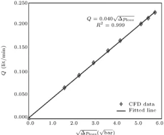
p in the orice, nozzle-apper and the lters were calculated by CFD method. It was revealed that the pressure drops in the lters and channels are negligible, compared to the orice and the nozzle-apper. In Figure 12, the variations of the ow versus pp is presented for the orice. The gure was obtained from simulating an axisymmetric model with CFD method. The uid ow was assumed to be turbulent, and K " model was used. Input and output pressures were applied as boundary conditions. In the case of the nozzle-apper, it is obvious that the distance between these two elements varies during the valve operation. Since the equilibrium distance is 0.06 mm for this sample valve, the ow-pp curve was plotted for few points in vicinity of this equilibrium distance. The required data in other internal distances are obtained by interpolation. These curves are shown in Figure 13. Details of the model are similar to the foregoing model of orice.
Figure 13. Flow values versuspp in various distances of the apper and nozzle.
SIMULATION
Equilibrium Angle of Flapper
As it was explained in previous sections, the apper displacement in terms of the input current was obtained by experiment (in the absence of the pilot hydraulic uid). However, in a real situation there is hydraulic pilot uid that ows from the nozzles to the apper. When the apper tilts towards each of the nozzles, a hydraulic force is exerted to the apper in the opposite direction, so its equilibrium angle is reduced. For calculation of this new angle, the following two steps should be done:
1. For initial guess, by means of Figure 8, the apper angle is calculated in terms of the input current in the absence of the uid forces by using xf= rf.
2. The calculated angle is then used for calculation of the components of Equation 19. If we set this equation as:
G = Tt Ts (F1 F2)r;
by trial and error, the f is found for G(f) = 0.
If G(f) > 0, then we reduce f and vice versa.
This process should be continued to nd the desired angle (f). According to Figure 5 and xf = rf the
xf is derived too.
Spool Displacement
As it is seen in Figures 12 and 13, the pressure drop in the orice and nozzle can be written as:
porice= C1Q0; (26)
where Q0 = Q2, C
1 is a constant and C2(xf) is a
function of xf (xf was derived previously so C2(xf)
can be derived from Figure 13). According to Figure 1, it is clear that the ow rate of the nozzle and orice in each side of the pilot circuit is equal. Also it was mentioned that the total pressure in the pilot circuit is 45 bar and the drain pressure is 7 bar. By neglecting the pressure drops in the lters and pipes it can be said that the whole pressure drop occurs in the orice and the nozzle-apper throats. As a result, one can say:
porice+ pnozzle= ptotal= 38: (28)
From Equations 26 to 28, Q0 can be written as:
Q0= ptotla
C1+ C2(xf) =
38
C1+ C2(xf): (29)
This process should be done for each side of the pilot circuit and a distinct ow rate is obtained for each nozzle. Now, it can be claimed that the pressures in the downstream of the two orices have been determined. In Figure 1 it is clear that the pressure behind each side of the spool is equal to downstream pressure of corre-sponding orice. Multiplying pressure dierence to the section area of the spool yields the resultant applied force to the spool in steady state condition. Since the stiness of the spool spring is known, the displacement can be calculated. The lapping phenomena can be then considered simply in this stage where the \port opening" (Po) is related to the spool displacement by:
Po= Sd lp
8 > < > :
lp> 0 overlapped
lp= 0 critically
lp< 0 underlapped
(30) where Po is the port opening, Sd is the spool
displacement and lp is the lapping of the spool and
port. If Po < 0, the port has not opened yet. In the
studied valve, 0.005 mm< lp< 0:01 mm.
All processes in this section are simulated using a computer based algorithm where the input is the current and the output is the control port opening. The spool displacement versus the input current is shown in Figure 14.
Output Flow
As it is seen in Figure 15, the spool displacement controls the output ow of the valve. In fact, the spool and the ports (machined on the spool body) are used as a variable orice. In Figure 1, it is obvious that the displacement of the spool is controlled by the pressure dierence between two sides of the spool which is due to the apper movement between the two nozzles.
Figure 14. Spool displacement versus the input current.
Figure 15. Section of the spool body and ports (spool has moved to the right from its equilibrium position).
According to Figures 1 and 15, this sample valve has two types of ports. One is the control port (such as ports P and Tank in Figure 1) that is used as a variable orice and its opening is proportional to the spool movement. The other type is used to direct the ow towards the actuator or from it (such as ports A and B in Figure 1). These ports are not controlled proportionally. Therefore, for modeling of the spool and ports, by paying attention to Fiuregs 1 and 15, a model such as the one shown in Figure 16 is proposed. Also in this gure, boundary conditions which are used in CFD modeling are shown. The model is axisymmetric. Pressure boundary conditions were
Figure 16. The CFD model of the spool body and the ports along with the related Boundary Conditions (BC).
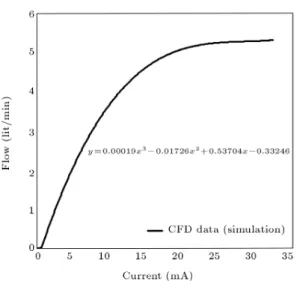
Figure 17. Simulated ow-current curve (dead zone, linear zone and saturation zone are seen).
applied and output ow rate was obtained. Fluid ow was assumed turbulent and K model was used for solving. This model was solved for various opening of the control port. Since the relation between the port opening and the input current was presented in Figure 14, the curve of the ow rate versus current is obtained in steady state condition. The recent curve is the main objective of this work. This graph is shown in Figure 17. The simulation is performed in a nominal supply pressure of 100 bar.
Summary of Simulation
- Flapper displacement is derived from Figure 8 for an arbitrary input current (0-35 mA). f = xrf is the
initial guess for the angle which is used for solving Equation 19.
- Equation 19 was then solved by trial and error (Tt
was obtained from Equation 20, Ts is obtained from
Ts= Ksf and `F1 F2' is derived from Figure 11).
- The ow rate of the nozzle and orice is derived by means of three algebraic Equations 26 to 28 in each side of the pilot circuit.
- The downstream pressure dierence of two orices was calculated. It is the same pressure dierence of the two sides of the spool (Figure 1). With the aid of spool spring stiness, spool displacement versus input current was obtained (Figure 14).
- Output ow is obtained by CFD method as discussed previously and shown in Figure 17.
EXPERIMENTAL RESULTS AND MODEL VALIDATION
For obtaining experimental data, a hydraulic tester was designed according to the SAE-ARP490 Rev E
Figure 18. (a) Front view of the hydraulic tester. (b) Side view of the hydraulic tester.
standard. In Figures 18a and 18b, two views of this hydraulic tester are seen. For ow measurement, a hydraulic jack and an encoder are used that is seen in Figure 18a. This jack can provide loading and unloading conditions. In this work, all tests were in unloading and steady state conditions. In order to provide pilot and load (supply) ow, two distinct pumps are used. The sample valve is set up on the tester and receives input current between 0 to 35 mA in 50 steps. The time of a complete course of the jack is measured. Then with the aid of cylinder dimensions (course: 90 cm and input diameter: 5 cm) and some calculations, the corresponding ow rate for each input current can be obtained. The pilot pressure is constant at 45 bar in each step and the variations of the load pressure from nominal pressure (100 bar) should be recorded. These recorded load pressures for each input current are used in ow simulation as boundary conditions.
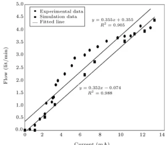
In Figure 19, the experimental data and the sim-ulated curve are compared according to four following principal variables:
- Flow gain: Flow gain is the slope of the linear zone of the ow-current curve. This zone is one of the most important characteristics of a ow control valve. In Figure 20, the calculated ow gain from the experimental and simulated data are compared. According to this gure, experimental gain is 0.355 and simulated gain is 0.352 (0.85% error).
- Saturation ow: According to Figure 19, it can be said that the experimental and simulated data show the ow saturation to happen at about 5 Lit/Min. - Saturation current: The saturation current is
cor-responding current of the saturation ow. According to Figure 19, it can be said that for both of them, the ow is saturated at about 20 mA.
Table 1. Experimental and simulation results. Flow Gain
(lit/Min.mA)
Saturation Flow (lit/mA)
Saturation Current (mA)
Dead Zone (mA)
Experiment 0.355 5 20 0
Simulation 0.352 5 20 1
Error 0.85% 0 0 1
Figure 19. Simulated results versus the experimental data for the ow-current curve in steady state conditions.
Figure 20. Simulated and experimental ow gain.
the spool and the ports. Since the lapping of this sample valve is measured to be about +0.01 mm, it is expected that a dead zone exists in the ow-current curve. This zone in the simulated curve is seen to be up to 1 mA. However, it is not seen in the experimental results. As the lapping of the spool and the port is very critical, sensing of this
zone in the ow-current test requires more accurate equipment.
Source of Errors
As the ow-current curve is the nal stage in the simulation of the valve behavior, it can be said that all errors of the previous stages appear in this stage too. Also some simplications such as neglecting the pressure drop in the lters and pipes contributed to the error. However, it seems that neglecting the friction between the cylinder and the piston of the jack and the piston inertia may be the most important sources of error.
CONCLUSION
In this work, the ow-current characteristic of a sample electro-hydraulic servo valve was simulated. Also a hydraulic tester was constructed to test some behaviors of the valve experimentally. The model incorporates all components of the valve (rst and second stage). The experimental and simulation results were compared for four important variables in Table 1. According to Table 1, the valve has a sucient accuracy. As a result, the model can be used for other studies such as sensitivity analysis. Using this approach, modeling of underlapped, critical center (zerolapped) and overlapped valves can be done in similar studies. ACKNOWLEDGMENT
The authors would like to express thanks to M. Gheis-ari for his helps in torque motor modeling, and M. Hemmati for his helps in the CFD analysis. Thanks to M. Karimi and H. Farajian Zade for their various helps. The experiments are supported nancially by Moje-Pouya Inc.
NOMENCLATURE
E electrical potential
N turns of coil
i electrical current
magnetic ux
k equilibrium distance of armature and body (equilibrium gap)
x displacement of the armature end 0 magnetic permeability of air
r relative magnetic permeability of the
substance
A area normal to the ux path in the air gap
B magnetic ux density
w electromagnetic energy
f armature force
Tt the produced torque by torque motor
Ts resistance torque of the exure tube
F pilot uid force
r radius of the apper from pivot to pilot uid forces
J polar mass moment of inertia of the apper and armature
c damping coecient of armature and apper
f rotation angle of the apper
xf apper displacement
Ks stiness of the exure tube
La Arm length of the armature
L equilibrium distance between the nozzle and the apper (L = 0:06 mm)
p pressure dierence
Po port opening
Sd spool displacement
lp lapping of the spool and the port
REFERENCES
1. Tawc, M.N. \Model based control of an electro-hydraulic servo valve", PhD Thesis, University of Akron, Akron-Ohio, US (1999).
2. Eryilmaz, B. and Wilson, B.H. \Unied modeling and analysis of a proportional valve", J. Franklin Institute, 343, pp. 48-68 (2000).
3. Johnson, J.L. \So what is the dierence between a proportional valve and a servo valve", J. Hydraulics & Pneumatics, 55(9), pp. 24-26 (2002).
4. Merritt, H.E., Hydraulic Control Systems, John Wiley and Sons, New York, US (1967).
5. Mookherjee, S. \Design and sensitivity analysis of a single-stage electro-hydraulic servo valve", Proc. of 1st FPNI-PhD Symp., Hamburg, Germany, pp. 71-88 (2000).
6. Kim, D.H. and Tsao, T.C. \A linearized electro-hydraulic servo valve model for valve dynamics sensi-tivity analysis and control system", J. ASME DSMC, 122, pp. 179-187 (2000).
7. Noah, D.M., Hydraulic Control Systems, John Wiley and Sons, New York, US (2005).
8. Amirante, R. et al. \Evaluation of the ow forces on an open center-directional control valve by means of a computational uid dynamic analysis", J. Energy Con-version and Management, 47, pp. 1748-1760 (2006). 9. Del Vescovo, G. and Lippolis, A. \CFD analysis
of ow forces on spool valves", 1st Int. Conf. on Computational Methods in Fluid Power Technology, Melbourne, Australia (2003).
10. Cheng, D.K., Field and Wave Electromagnetics, 2nd Ed., Addison-Wesley, Massachusetts, US (1989). 11. Walters, R.B., Hydraulic and Electro-Hydraulic
Con-trol Systems, ELSEVIER Science Publisher LTD (1991).
BIOGRAPHIES
Mohammad Saleh Sadooghi received his B.S. de-gree from Sharif University of Technology in Tehran, I.R. Iran and his M.S. degree from Bu-Ali Sina Uni-versity in Hamedan, I.R. Iran, in Applied Mechanics, in 2008. He is now a teacher of robotics engineering at Hamedan University of Technology. His favorite research is Modeling of Electro-Hydraulic Systems as well as Robotic Systems in Vehicles.
Rahman Sei received his Ph.D. degree in Mechanical Engineering in 2004 from the University of Tarbiat Modarres, Tehran, I.R. Iran. He is now a faculty member of mechanical engineering at Bu-Ali Sina University in Hamedan where he teaches courses at the `Applied Design group' of the Mechanical Engineer-ing Department. His teachEngineer-ing focuses on Automatic Control, Strength of Material, Fracture Mechanics at undergraduate and graduate levels. Dr Sei has also published 6 articles in international journals and about 50 conference papers.
Mahmoud Saadat Foumani received his Ph.D. de-gree in Mechanical Engineering from Sharif University of Technology, Tehran, I.R. Iran, in 2002. He was a Faculty member at Semnan University from 2002 to 2006 and is now a faculty member of Sharif University of Technology, Mechanical Engineering Department. He teaches courses at the `Applied Design group' at un-dergraduate and graduate levels. His teaching focuses on Mechanical Engineering Design, Vehicle Dynamics and Chassis Design and Advanced Mathematics.