World City Mode Choice: Choice
of Rail Public Transportation
H. Poorzahedy
, N. Tabatabaee
1, M. Kermanshah
1,
H.Z. Aashtiani
1and S. Toobaei
2The choice of technology to transport passengers in large metropolitan areas is an important issue everywhere. There are many factors involved in this choice. This paper deals with the possibility of the objective use of available information in the analysis of the suitability of a rail public transport system for a city. A database has been made from publications on public city transportation and country level information. Logit models of choice have been calibrated by the maximum likelihood and nonlinear least square methods based on the acquired information. Each city is treated as an \individual", choosing rail or non-rail modes for its trips. Only cities with a population of more than one million have been included in the analysis to ensure the instigation of mode diversication in these cities. Selected models have been validated and then used to suggest the desirability of a rail public transport mode in some sample cities, according to world practice.
INTRODUCTION
The choice of technology for the movement of pas-sengers in large metropolitan areas, particularly in developing countries, poses some dicult questions for transportation authorities in many of these population centers. On the one hand, increasing demand for transportation, deteriorating urban environments and tension caused by trac and congestion and, on the other hand, deteriorating transportation systems and the lack of resources to upgrade these systems may make one conclude that high investment options are the only solution to ever-rising transportation prob-lems. This makes the issue a nancial one for those responsible.
Questions facing authorities may include:
Does the city need a high-cost transportation
sys-tem, such as rail transportation?
What proportion of rail/non-rail mass
transporta-tion is appropriate for the city?
*. Corresponding Author, Department of Civil Engineering, Sharif University of Technology, Tehran, I.R. Iran.
1. Department of Civil Engineering, Sharif University of Technology, Tehran, I.R. Iran.
2. Department of Civil Engineering, University of Mary-land, College Park, MD, USA.
What spectrum of public transportation systems
(various types of buses and light and heavy rail transit) is suitable for the city?
What are the appropriate market shares for the
modes in this spectrum?
These are very dicult questions to answer for a multi-tude of reasons. One is the perceived need for high-cost alternatives (e.g., rail transport systems) stemming from a rapid increase in transportation demand and amplied by a deteriorating environment, including air pollution, largely caused by the use of fossil fuels and out-dated motor vehicles. High-cost transportation alternatives, believed to have a high capacity and which enjoy clean technologies, seem appropriate to solve the above-mentioned problems.
Another reason is the inherent complexity of problems stemming from many other sources, as fol-lows. One is the existence of multiple objectives linked with the interests of diverse groups, which makes the problem controversial and political in nature. Another is that eective mass transportation technologies are very expensive and the resources available to these large cities are very limited. Government subsidies may already account for a substantial portion of the public transport budget, so that local and central governments are no longer potentially and/or politically able to
un-dergo further major expenses in this regard. Moreover, sources of non-government, or tax or toll-based funds in many third world countries are very limited for dierent reasons. Existing tax laws may be out-dated or ill-dened (an example is where taxes are collected from producers rather than consumers) and the legislative mechanisms in these countries may be plagued with political and administrative complexities.
For most developing countries, new transporta-tion technologies are imported from industrialized countries. Authorities in developing countries en-counter the added diculty of nancing the new systems with foreign currencies, a precious resource to many of them.
Finally, a shortage of information and data, tools for analysis and experts are other complex aspects to the problem of choosing an appropriate technology for eective mass transportation in large metropolitan cities in many developing countries. These diculties make the decision-makers choose subjectively when an opportunity to invest in a new transportation system appears. As a result, such decisions are apt to involve errors.
There is numerous literature regarding public transportation analysis and planning; [1-3] are exam-ples of texts covering various aspects of public trans-portation planning and technology, which also present many related references. Banister and Pickup [4] present another bibliography in this area. The con-ference proceedings published by the Institution of Civil Engineers [5,6] present many research papers on the issue of rail public transportation. Some authors (e.g. [7]) try to sketch the situation where a rail transit system becomes successful. Recently, Parajuli and Wirasinghe [8] presented a decision analytic model for the selection of mass transit technology in a transit corridor with a known right-of-way category and rules of operation. They, basically, attempt to analyze (various aspects of) the problem of public transport technology choice. However, because of the complexi-ties mentioned above (as well as others not mentioned), it is unfortunate that it is not an easy task to nd out when a rail public transport system does suit a city.
One way to help the decision-making bodies of large cities in their choice of alternative transportation technologies is to inform them of the decisions of others in similar situations. Many large cities have made these choices in the past century as their systems deteriorated, became obsolete and demand changed spatially and temporally. They now possess a wide range of systems to serve their needs. One can consider a city (including its citizens, interest groups and various governmental and decision-making bodies) to be an \individual" who chooses modes to make trips. The decisions of these individuals can be used
to build a model of mode choice, which describes the choice of modes (technologies) as a function of the characteristics of the cities (individuals), attributes of the technologies (modes) and peculiarities of the countries (environment) to which they belong. In eect, such a model is a condensed \expert" system.
The main purpose of this paper is to propose a means to aid the decision maker in adopting rail transit. Furthermore, it can be used by rail transit system providers to demonstrate the potential of cities that can benet from such systems. To this end, this study employs Jane's Urban Transport Systems [9] as the source of transportation data for the cities and the United Nations Report on Human Development [10] as the source of socio-economic characteristics of the respective countries, to create a database for the choice of technologies (mode of transportation) by the representatives (of the citizens) of large cities in the world. The information collected will form a base for an objective analysis of the choice problem and will be used to calibrate a mode choice model to show whether or not the common practice of world cities would candidate a city with given characteristics for a rail transportation system. Some models will be presented, calibrated, validated and used to suggest the choice of non-rail or rail + non-rail options to serve a city's transportation needs. The data base used in this study may suggest the type of information that is essential for some choice analyses and, hence, may be used as a guide for various organized eorts in data collection in this area.
DATABASE CHARACTERISTICS
General Database
There are some organizations that collect and period-ically report data on various aspects of the modes of transportation available in large cities around the world (e.g. [9,11]). The collected information, however, varies among references and includes the overall characteris-tics of the city (population, area, etc.), various public transportation modes, a basic description of these modes (annual vehicle-kilometers, etc.), fare structure of the modes, working hours, sources of funds and a detailed description of vehicles (number of seats, passenger capacity, etc.).
One diculty in using these data is that not all of the items are clearly dened, nor are the questions always accurately answered by the transportation au-thorities of the participating cities. It should also be added that there are considerable data missing from the above compilations. Another diculty is that data from various sources may not be put together to en-hance the quality of data (cross checks, lling in missing information, etc.), or widen the range of information
Table1. Content of database for an analysis of public transportation technology needs.
Information Category
Main
Bus, Trolley
Bus, Other
Non-Rail
Tramway, LRT,
Metro
Minibus,
Taxi
Row no.
Identity Country name Row no. Row no. Row no.
City name
City characteristics Greater city pop (mil)City population (mil.) Real GDP/capita1
Adjusted GDP/capita1
Country GDP index1
characteristics Human dev. index1
Degree of industrialization2
Political system3
Public transportation trips
(millions/year)
All modes, 1987 All modes, 1988 All modes, 1989
1987 gure 1988 gure 1989 gure
1987 gure 1988 gure
1989 gure Yearly g. Vehicle-kilometers
(millions/year)
1987 gure 1988 gure 1989 gure
1987 gure 1988 gure
1989 gure Yearly g.
Network No. of lines No. of routes
characteristics Total route length Total route length No. of stops
Vehicle
characteristics Vehicle capacityNo. of vehicles
Headway, pk.
Service Headway, o pk.
characteristics lst train time
Last train time Flat
Fare structure Regional
Distance-based
Operating cost Subsidies Subsidies
Financial sources Commercial Commercial
Fare Fare
Others
1. See [10] for denition; 2. Industrialized equals 1, otherwise 0; 3. Formerly socialist equals 1, otherwise 0.
(across attributes or subjects), because they dier in the denition of terms or belong to dierent years. Also, some relevant information for objective analyses of such data has not been collected. The aim of the collecting organizations seems to be to give an overall picture of the transportation infrastructure of the large cities of the world for qualitative and comparative
analyses of their transportation systems or for a study of the transport technologies themselves.
Employing Jane's Urban Transport Systems [9] as the source of transportation data, only large urban areas with a population of 1 million and over are considered to ensure the diversity of modes within a city and the need for various modes. Table 1 shows the
type of information included in the database for each mode.
To reduce the number of missing values for the subject cities, data spanning the years 1987 to 1989 have been considered. The data show very little change in these consecutive years, thus, they can correct themselves and their average values can be a good estimate of the respective yearly gures. For the few cities with missing values in these three years, the available values in the nearest year have been considered. One hundred and seventy four cities were selected for the construction of this data set.
The socio-economic characteristics of the coun-tries of the selected cities, from the United Nations Report on Human Development for 1992 [10], belongs to a year close to our 1987-89 statistics for trips. Other reports in this series were consulted for the cases which lacked information. The data were added to the \main" table, which was augmented by two other items of information: \degree of industrialization" and \political system". The items in the database are shown in Table 2.
Rail/Non-Rail Database
To address what share of the trips made in a large city is given to rail public transport systems by the city authorities, a database of mode choice by a city was created with the following specications. For modes containing data for all three years from 1987-89, an
average gure was computed as a representative value of that information item (e.g., yearly trips made by that mode). Cities with no values for any of the modes were discarded. Also, trips reported for several companies operating in a specic mode (e.g., bus companies) in one city were added together to form the total trips made by that mode. The case (city data) was omitted if ambiguities existed for the data. For minibuses and taxis (minibus-taxi), data were rough estimates of percentage. Where the information could be translated into yearly trips, the case was included in the data-base, otherwise it was omitted.
The trips made by the rail modes were summed together, as were those of non-rail modes. Rail and non-rail trips were then added together to build two super modes: \rail" (rail + non-rail) and \non-rail", for each city (denoted byr and n, respectively). The
database thus created includes the information items shown in Table 2. This database contains 126 records for 126 cities with populations of over 1 million.
MODEL FORMULATION
As mentioned before, one may consider each city as an \individual" who is making a choice of its mode of transportation. In this concept, the transportation authorities and the users of the facilities are considered elements of one entity deciding to make some modes available to itself, as well as deciding how often to use which mode. Suppose that the then decision to
Table2. Database for analysis of rail/non-rail choice.
Information
Item in
Database
Denition
Equivalent
Variable
in Models
Row
Subject ID numberPopl
City population, millions of population in1989 PPoph
Greater city population, millions, in1989 p gPas-rail
Passenger trips made by rail public transport, billions/year in1989 T rTotal-pas
Total passenger trips by rail and non-rail public transport, T tbillions/yr in1989
Pas-popl
Pas-poph
\Total-pas"/\pop-h" (x100)\Total-pas"/\pop-1"(x100)tpp tpp
g
Railexist
If pas-rail>0 (existence of rail mode) = 1, otherwise = 0 yRgdp
Real GDP per capita (ppp $1000) in 1992 GAd-gdp
Adjusted real GDP per capita ($1000) AGHdi
Human development index hdiPol
Formerly socialist countries = 1, otherwise = 0 polIndst
Industrialized countries = 1, otherwise = 0 indhave a rail system is the current such decision (this is generally true and, hence, it does not seem to be basically a binding assumption). It will be assumed that the underlying rule of choice follows a logit model as follows [12]:
p r= e ur e u r+ e u n = 1 1 +e
(ur un)
; (1)
p n= 1
p r
; (2)
where p
r is the probability that the \individual"
chooses to have both rail and non-rail modes of trans-portation, as opposed to p
n, where it chooses only
non-rail modes. It is assumed that the modes of transportation existing in the city will be among the current choices. It is also assumed that all cities have had some form of non-rail transportation (e.g., bus) before having a rail transportation system. In this sense, p
r is equivalent to the probability of having a
rail system.
It is clear from Equation 1 that p
r and, hence, p
n, are only functions of the relative utilities of the
two states,u r
u
n, rather than their absolute values.
Moreover, it can also be concluded from Equations 1 and 2 that the ratio of the probabilities of the two states (rail/non-rail), usually referred to as relative odds [12], is: p r p n =e u r u n : (3)
So that, again, it is the relative utility functions which govern the ratio. Equations 1 and 3 convey the notion that, to specify the utility functions of the states, it is sucient to dene them as follows (assuming an additive utility function):
u r= k 1 X j=1 j f j( x j) ; (4) u n= k ; (5) wherex
js are the choice descriptive variables and
js
(j = 1;2;:::;k) are parameters of the utility functions
(to be calibrated).
Model Calibration
Maximum Likelihood Estimation Method
By assuming that the decision of public transport technology in one city is independent of those in other cities, the contribution of city i to the logarithm oflikelihood function,L (
i), is dened as: L
( i) =y
iln( p
r(
i)) + (1 y i)ln(1
p r(
i)); (6)
where y
i takes the value of 1, if city
i has both rail
and non-rail public transport systems and 0 otherwise. Then, the logarithm of likelihood function, L
, would
be computed as:
L = N X i=1 L (
i); (7)
whereN is the number of cases under study (here, 126).
Thus, if cityihas both rail and non-rail systems, then y
i = 1 and 1 y
i = 0 and the contributing portion
of Equation 6 becomes ln(p r(
i)). Otherwise y i = 0
and Equation 6 contributes ln(1 p r(
i)), which equals
ln(p n(
i)).
Maximizing the objective function, Equation 7, with respect to the
js and using an appropriate
statistical optimization package, such as GAUSS [13], gives the estimated parameters of the utility functions, based on the maximum likelihood criterion. Many models with dierent utility functions have been cal-ibrated and tested, among which three formulations have been chosen as the \best" models, based on the following criteria: (a) The estimated parameters are signicantly dierent from zero, at least at the 95% condence level; (b) The parameters have the correct signs (i.e., as expected or interpretable); and (c) The analog of R
2 (coecient of determination) in least
square estimation,
2, as dened below, has the highest
value among the calibrated models:
2= 1
L ( )=L (0) ; (8) where L (
) and L
(0) are the (negative of)
log-likelihood function at the estimated values of the parameter vector and at = 0, respectively. The
former carries the power of the calibrated model in representing data and the latter shows that of the no information (equally likely alternatives) case. Thus,
2
shows the percent improvement in the log-likelihood value of the calibrated model, as compared with that for the no-information case (with equal probability for the two alternatives). The selected models mentioned above are given in Table 3 as models ML1 to ML3.
Nonlinear Regression Approach
Some of the superior models calibrated by the max-imum likelihood method are recalibrated using the method of nonlinear regression, minimizing the sum of squared errors. The results are shown in Table 3, as models NLS1 to NLS3.
As may be seen in Table 3, rescaling the parame-ters [14] of models NLS1 and NLS2 with the objective of having identical constant parameters, as in those of models ML1 and ML2, respectively, yields similar parameters to those of ML1 and ML2.
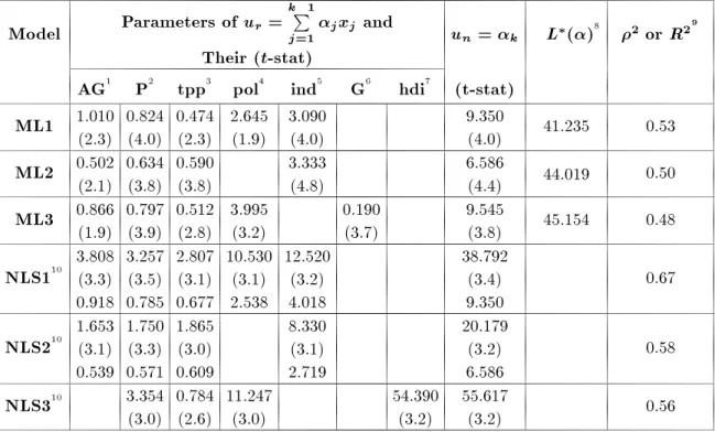
Table3. Selected models for the choice of rail/non-rail public transportation in large cities.
Model
Parameters of
u r=
k 1 P j=1
j
x j
and
Their (
t-stat)
u n
=
k
L
(
)
82
or
R 2
9
AG
1P
2tpp
3pol
4ind
5G
6hdi
7(t-stat)
ML1
1.010(2.3) 0.824(4.0) 0.474(2.3) 2.645(1.9) 3.090(4.0) 9.350(4.0) 41.235 0.53ML2
0.502(2.1) 0.634(3.8) 0.590(3.8) 3.333(4.8) 6.586(4.4) 44.019 0.50ML3
0.866(1.9) 0.797(3.9) 0.512(2.8) 3.995(3.2) 0.190(3.7) 9.545(3.8) 45.154 0.48NLS1
103.808 (3.3) 0.918
3.257 (3.5) 0.785
2.807 (3.1) 0.677
10.530 (3.1) 2.538
12.520 (3.2) 4.018
38.792 (3.4)
9.350 0.67
NLS2
101.653 (3.1) 0.539
1.750 (3.3) 0.571
1.865 (3.0) 0.609
8.330 (3.1) 2.719
20.179 (3.2)
6.586 0.58
NLS3
10 3.354(3.0) 0.784(2.6) 11.247(3.0) 54.390(3.2) 55.617(3.2) 0.56
1. AG: Adjusted real GDP per capita; 2. P = City population; 3. tpp = Per capita public passengers per year; 4. pol = Political system of the country; 5. ind = Industrialized status of the country; 6. G = Real GDP per capita; 7. hdi = Human development index; 8.L
(0) = 88 :34; 9.
2is a goodness-of-t measure for maximum likelihood method, and R
2 for nonlinear least square method. 10. Figures in the third row are rescaled values of parameters.
Evaluation of Models
Table 3 shows that models ML1 and NLS1 possess bet-ter goodness-of-t values than those of their respective counterparts. Table 4 shows some characteristics of the predictions of models ML1 to ML3 in Table 3. The same information for models NLS1 to NLS3 are given in Table 5. The correlation matrix in Table 4 shows that there is a strong association between the existence (or non-existence) of rail in a city (y) and the
probability that the city has a rail (and non-rail) public transportation system (p
r), as predicted by a model.
Higher correlations exist between the predictions of these models themselves. This is expected, since y
is integer-valued (i.e., it has a value of 0 or 1) while its prediction is real-valued (between 0 and 1). Of the three models in Table 4, prediction results for model ML1 show higher correlation with y (0.7841)
and indicate a lower mean for probability, p
r, when
there is no rail in the city (0.217). They present a higher value for it when the city, in addition to non-rail urban transportation technology, also has a rail system (0.815). The standard deviations ofp
rvalues for y= 0
and 1 in Table 4 also show more stable predictions for
model ML1 relative to the other two models (ML2 and ML3).
Table 5 shows characteristics similar to model ML1 for model NLS1, compared to the others. How-ever, model NLS1 shows stronger values for the above-mentioned statistics than model ML1; itsp
rpredicted
correlation with y is 0.8264 (instead of 0.7841 in the
case of model ML1), with a mean p
r for cases having
non-rail and rail modes equal to 0.126 and 0.887 (instead of 0.217 and 0.815), respectively. On the other hand, model NLS1 shows slightly higher standard deviations for its probability, p
r, for the two cases of y = 0 and 1, than does model ML1. This is also
true for models ML2 and NLS2, which are the same, but calibrated by dierent methods. Hence, Tables 4 and 5 show that models calibrated by the nonlinear regression method (NLS) predict closer to the two extreme values of 0 and 1, but with higher dispersion (standard deviation).
Figure 1 shows the probability for the choice of rail (p
r) in the cities under study for rail ( y = 1)
and non-rail (y = 0) modes, as predicted by models
ML1 to ML3, which are calibrated by a maximum likelihood procedure. The gure indicates predicted
Table4. Some characteristics of the predictions made by ML1 to ML3.
Information
Information Item
pr
No. of
Category
ML1
ML2
ML3
Observ.
y# 0.7841 0.7544 0.7553
Correlation
pr, ML1 1.0000 0.9761 0.9499
Matrix
pr, ML1 1.0000 0.9167 126
p
r, ML1 1.0000
p
r Mean 0.217 0.236 0.243
Statistics
Std. Dev. 0.263 0.273 0.263for Cases
Minimum 0.001 0.007 0.008 58Where
y= 0
Maximum 0.990 0.955 0.997SEE 1.212 1.157
p
r Mean 0.815 0.799 0.793
Statistics
Std. Dev. 0.214 0.223 0.218for Cases
Minimum 0.076 0.102 0.069 68Where
y= 1
Maximum 1.000 0.9999 0.931SEE 0.263 0.279
#y= 1 (0) if rail does (not) exist in the city.
Table 5. Some characteristics of the predictions made by models NLS1 to NLS3.
Information
Information
pr
No. of
Category
Item
NLS1 NLS2 NLS3 Observ.
y # 0.8264 0.7723 0.7605
Correlation
pr, NLS1 1.0000 0.9496 0.9195
Matrix
pr, NLS2 1.0000 0.8851 126 p
r, NLS3 1.0000
p
r Mean 0.126 0.155 0.190
Statistics
Std. Dev. 0.268 0.280 0.317for Cases
Minimum 0.000 0.000 0.000 58Where
y= 0
Maximum 1.000 1.000 1.000SEE 2.127 1.806
p
r Mean 0.887 0.839 0.862
Statistics
Std. Dev. 0.255 0.285 0.261for Cases
Minimum 0.000 0.001 0.000 68Where
y= 1
Maximum 1.000 0.999 1.000SEE 0.287 0.340
#y= 1 if rail exists in the city, otherwisey= 0.
versus observed probability values (p
r). As may be seen
in this gure, for all three models, the probabilities of choosing rail are clustered in the higher values (i.e., closer to 1) for cases with existing rail transport and vice versa. Model ML1 performs better, in this sense, by predicting closer to 1.0/0.0 for cases where y = 1/0, than do the other two.
Figure 2 is similar to Figure 1, but for models NLS1 to NLS3, which are calibrated using the non-linear regression method. This gure shows that the models predict values of p
r much closer to 1.0/0.0 for
cases wherey= 1=0, compared to models ML1 to ML3
in Figure 1. (The number of observations is the same in both gures.)
Figures 3 and 4 show the information in Figures 1 and 2, respectively, in a frequency distribution form for the superior models ML1 and NLS1. As is evident from Figures 3 and 4, the frequency distributions are polarized for model NLS1 and more widely distributed for model ML1.
DISCUSSION
The merit of the Nonlinear Least Square (NLS) cali-brated models compared to those calicali-brated by Maxi-mum Likelihood (ML) is the higher correlation between predictions and observations,p
r, where
y= 1 and p n,
Figure1. Predictions of models ML1 to ML3, for the
choice of rail public transportation,pr, where rail mode
exists (y= 1) and where it does not (y= 0).
Figure2. Predictions of models NLS1 to NLS3, for the
choice of rail public transportation,p
r, where rail mode
exists (y= 1) and where it does not (y= 0).
method, total \distance" between the corresponding prediction and observation (sum of squared error) is minimized.) However, maximum likelihood models have other merits that deserve attention.
First, it should be noted that the ML method might be more appealing, theoretically, than NLS. This stems from the fact that the ML method is based on maximizing the probability of the joint occurrence of some (assumed independent) events, as opposed to the NLS method, which minimizes the sum of (squared) errors.
Second, it has been pointed out that, although ML estimates of the parameters cause the models to predict p
r a little farther from 1.0/0.0 for
y = 1=0,
the predictions are more consistent and have lower dispersions (standard deviation), when compared to the parameters obtained with the NLS method. In
Figure 3. Frequency distribution of the probability to
have rail (and non rail),p
r, as predicted by model ML1 for
cities with (a) no-rail and (b) rail public transport system.
fact, the standard error (standard deviation divided by mean) of the estimates (SEE) ofp
r, for cases where y = 1 andy = 0, is lower for the ML method than for
the NLS method, as shown in Tables 4 and 5.
Third, it can be shown that the direct (point) choice elasticities are as follows [14]:
E i(
x ik) = (
@p i
=p i)
=(@x ik
=x ik)
=x ik
:(@v i
=@x ik)
:(1 p i)
; (9)
where x ik is
kth variable in the utility function of the ith choice andE
i( x
ik) is the direct (point) elasticity of
choice of i with respect to x ik
: v
i is the deterministic
part of the utility function of alternativei, the partial
derivative of which, in Equation 9, is equal to ik, the
coecient ofx
ik, when v
i is a linear function of x
iks: E
i( x
ik) = x
ik
ik(1 p
i)
: (10)
Since the parameters of the NLS models in Table 3 are three to four times larger than those of the ML models, Equation 10 shows that ML models with lower
Figure4. Frequency distribution of the probability to
have rail (and non rail),p
r, as predicted by model NLS1
for cities with (a) no-rail and (b) public rail transport system.
ik's exhibit lower choice elasticity, with respect to the
variables in the utility function, compared to their NLS counterparts.
Finally, Tables 4 and 5 show that the correlation coecients for predictions between ML models are higher than those between NLS models. This means that, for the models at hand, the ML estimates of the parameters create models that are less aected by changes in variable specications. That is, ML models show higher stability in their predictions, so, if a variable is missing from the utility function, or vice versa, it will harm these models less.
MODEL PREDICTION
The models presented in this paper can be used to predict whether or not transportation authorities of a given city, with a population of over 1 million, will decide to add rail transportation to the existing non-rail modes, as would an \average" city. Two cities,E
andF, in a country with the following characteristics,
are considered. The country has an adjusted per capita GDP of $5,155 per year (AG = 5.155) and a human development index (hdi) of 0.77, which is non-socialist (pol = 0) and is not considered to be industrialized (ind = 0) in 1992. The available set of information pertinent to citiesEandF belongs to year 1994, the closest year
to year 1992 and includes the following:
1. Population: 6.8 and 2.03 million, respectively; 2. Estimated total public transport trips per year:
1,830 million and 535 million, respectively (T t =
1:83 and 0.535);
3. Total public transport trips per year per capita: 269.1 and 263.55, respectively (tpp = 2.691 and
2.6355).
Let us, now, consider model ML1 to suggest whether these two cities need public rail transportation, accord-ing to \world practice". The utilities of rail (rail + non-rail) and non-rail alternatives are U
E r = 12
:082
and U E n = 9
:350 for city E, resulting in p E r = 0
:939
for this city (Table 6). This is rather high, suggesting the need for a rail transport system according to such practices. Similar computations use U
F r = 8
:127 and U
F n = 9
:350 as the utilities of rail for city F, which
result inp F r = 0
:227.
Are these probabilities high enough to warrant the construction of a rail transportation system? To answer this question, Acceptance (A) and Rejection (R) Criteria (C) must be dened:
1. AC = The construction of a rail transport system is warranted, according to \world practice", ifp
r p
u;
2. RC = The construction of a rail transport system is not warranted, according to \world practice", if
p r
p l;
wherep u and
p
l are two pre-specied thresholds, with p
l p
u. A simple case would be where p
l = p
u =
0:5. If the value ofp
r for a city i, p
i
r, is less than 0.5
(or greater than or equal to 0.5) one would reject (or accept) the construction of a rail system for that city. A more rigorously dened value of the thresholds may be obtained as follows:
A set of cases in the data-set with rail transport
systems, i.e., withy = 1;
R set of cases in the data-set with no rail system,
i.e., withy= 0;
Table6. Model suggestion for building a rail transportation system in sample citiesE andF.
Decision
City Model Case Description
U rU n
p r
p n
p 1
= 0
:
217
pu
= 0
:815
ML1 Base case 8.127 9.350 0.227 0.773 Indecisive(
No)
ML1 Population increase 9.354 9.350 0.501 0.499 Indecisive to 3.52 million
ML1 Adj. real GDP increase 13.080 9.350 0.977 0.023 Yes to $7000 & ind = 1
ML1 Country become 11.217 9.350 0.866 0.134 Yes industrial: ind = 1
F ML1
City in a socialist
country: pol = 1 10.772 9.350 0.806 0.194 Indecisive(Yes)
ML2 Base case 5.428 6.586 0.239 0.761 Indecisive(
No)
ML3 Base case 5.458 9.545 0.252 0.748 Indecisive(
No)
NLS1 Base case 33.640 38.792 0.006 0.994 No NLS2 Base case 16.986 20.179 0.039 0.961 No NLS3 Base case 50.754 55.617 0.008 0.992 No ML1 Base case 12.082 9.350 0.939 0.061 Yes ML2 Base case 8.485 6.586 0.870 0.130 Yes ML3 Base case 12.287 9.545 0.940 0.061 Yes
E NLS1 Base case 49.179 38.792 0.99997 0.00003 Yes
NLS2 Base case 25.436 20.179 0.9948 0.0052 Yes NLS3 Base case 66.796 55.617 0.999986 0.000014 Yes
* Yes = Build; No = Do not build, Yes = Almost Yes,No = Almost No,
Indecisive = Further investigations are needed to reach a conclusion. n
A= jAj; n
R= jR j; p
u= f(p
i r
;i2A); (11)
p l=
g(p i r
;i2R); (12)
where:
n A+
n R=
n; (13)
and where f(:) and g(:) are two functions of the
probabilities of choosing a rail system for some cases in the data-set,AandR, respectively, as predicted by
a choice model, such as model ML1. The following average functions forf(:) andg(:) will be used in this
paper:
p u= 1
n A
X i2A p
i r
; (14)
p l= 1
n R
X i2R p
i r
: (15)
It is clear that, for p l
p
u, there may be an area
of indecisiveness, where p l
< p i r
< p
u, in which case,
one may neither accept nor reject the need for a rail transport system for cityi.
For the data set at hand, based on the predictions of model ML1, p
l = 0
:217 and p u = 0
:815 and then
based on the values ofp E r and
p F
r computed above, one
may say:
p E r = 0
:939 > 0:815, where construction of rail
transportation is warranted for cityE; 0:217< p
F r = 0
:227 < 0:815, where no conclusion
may be reached on construction of a rail system in cityF.
In fact, a closer look at the p
r values shows that city E has a p
r value greater than those of 56 out of 58
system (Figure 3a). Moreover, the value ofp
rfor city E
is greater than that of 40 out of 68 cities (59%), which have some type of rail transit system (Figure 3b). The
p
rvalue for city
Fis greater than that of 40 cities with
no rail (69%), but greater than that of only 3 cities with rail (3%) (see Figures 3a and 3b). That is, city
E is doing much better than most others that do not
have rail and better than 50% of those that have rail and, hence, probably needs a rail transport system. By contrast, cityF is doing better than 50% of cities with
no rail, but much worse than those with a rail system. Thus, based on the information at hand, it is dicult to predict whether or not it needs a rail system according to \world practice".
Table 6 presents the suggestions made by various models for the construction of rail transport systems for cities E and F. These are identied as \base
cases" in this table. As may be seen in Table 6, models ML1 to ML3 present consistent values forp
r,
as do models NLS1 to NLS3, for each city. However, values for p
r, given by models NLS1 to NLS3, are
substantially lower than those given by models ML1 to ML3 for cityF, whereas the reverse is true for city E. That is, models NLS1 to NLS3 predict in extremes,
as mentioned before, easily rejecting a rail option for cityF and accepting it for cityE. It seems as though
the NLS method of calibration has some sort of internal mechanism that demands a decision for a given case.
SENSITIVITY ANALYSIS
It is instructive to nd out under what circumstances would an indecisive situation turn into a denitive one. Likewise for other factors, what changes in some attributes of city F turn its indecisive situation into
a clear positive signal for the construction of a rail system. Table 6 shows the eect of some of these changes upon the choice of technology in cityF.
If city F were experiencing a high rate of
popu-lation growth because of high in-migration, what level of city population would warrant construction of a rail system? Assuming a more liberal value ofp
u= 0 :5 for
an AC, from Equation 1, one should have:
p r=
1 1 +e
u n
u r
p u= 0
:5; (16)
or:
u n
u r
0: (17)
From model ML1 in Table 3, it can be shown that:
P3:52 million people. (18)
If the estimated population for 20 years from now is approximately at this level, one may suggest a rail transport system for city F now, owing to the fact
that it usually takes 5-10 years to build such systems, particularly in developing countries.
If city F is in an industrialized country with an
adjusted per capita GDP of around $7000 (instead of $5155 value), then, all else being the same,p
F r = 0
:977,
warranting a rail system. The value of p F r, with
the original adjusted GDP value in an industrialized country, would become 0.866, suggesting the same conclusion.
Even if cityF was in a formerly socialist country,
all else being the same,p F
r takes a value equal to 0.806,
barely justifying the existence of a rail system in this city, according to average practice in world cities.
CONCLUSIONS
The purpose of this paper was to propose a concept for a decision-maker facing a decision about the need for a rail public transport system for a city, information regarding the average practice of world cities. The cities of 1 million population and over in the world are envisaged as \individuals" that are selecting modes of travel.
To this end, a data set was created. This data set is neither complete in variables, nor exhaustive in cases. It is an example of how to bring together some of the already collected data by various organizations. A binary logit model is proposed to model the choice of mode (technology) for a city. Several models have been proposed and calibrated by two methods, the method of Maximum Likelihood (ML) and the Nonlinear Least Square method (NLS) and, then, validated according to various statistics.
The selected models have been used to describe the need for a rail mode for two sample cities, as well as to perform a sensitivity analysis for a non-decisive case. Based on the calibrated models, it is found that:
The NLS model predictions are closer to the two
extreme values of probability range [0,1],
The NLS models predicted with wider dispersion
(standard deviation),
The standard error of estimates of ML models is
lower, which implies more consistent predictions by these models,
ML models with lower utility parameter values
exhibit lower choice elasticity with the utility func-tion variables, which reduces the risk of erratic predictions,
ML models showed higher correlation coecients for
their respective predictions.
It is very important to emphasize that the models presented in this paper are intended to condense world practice in introducing rail transport systems to large
cities. They should be viewed as some tools for convey-ing such information and are, by no means, designed to imply a nal \yes" or \no" to the construction of a rail transport system in a city.
The choice of rail transportation is a multi-objective decision. It would be nave to think other-wise. However, one may place a weight of nearly 100% on a single objective, e.g., \creating the image of a modern city" to decide to build it, or see it in deance of personal freedom to decide against its construction. Such singularities, or other possibly irrational decisions in this regard, may be captured by the random part of the utility of the decision.
Future research directions may include enhance-ment of data in dimensions such as geography and the shape of the city.
ACKNOWLEDGMENTS
This paper is part of the research project conducted by the authors for Mashad Transportation Planning Au-thorities. The authors greatly appreciate the support provided. They also wish to thank Mr. Amir-Reza Mamdoohi for his technical assistance in computer programming and running the computer programs.
REFERENCES
1. Gray, G.E. and Hoel, L.A., Public Transportation: Planning, Operations and Management, Prentice-Hall, New Jersey, USA (1979).
2. Vuchic, V.R., Urban Public Transportation: Sys-tems and Technology, Prentice-Hall, New Jersey, USA (1981).
3. Black, A., Urban Mass Transportation Planning, McGraw-Hill, Inc., New York, USA (1995).
4. Banister, D. and Pickup, L., Urban Transport and
Planning, A Bibliography with Abstracts, Mansell Publishing, Ltd., London, UK (1989).
5. The Institution of Civil Engineers \Rail mass transit for developing countries", Proceedings of the Confer-ence, London, 9-10 October 1989, Thomas Telford, London, UK (1990).
6. The Institution of Civil Engineers \Light transit sys-tems",Proceedings of the Symposium on the Potential of Light Transit Systems in British Cities, Notting-ham, 14-15 March 1990, Thomas Telford, London, UK (1990).
7. Schumacher, R. \What kind of rail transit system?- for a city or region that does not now have rail transit", Kent, L.B. and Jones, D.L., Eds., Transportation Congress: Civil Engineers-Key to the World's infras-tructure, Proceedings of the 1995 Conference, San Diego, CA, ASCE, pp 1468-1478 (Oct. 22-26 1995). 8. Parajuli, P.M. and Wirasinghe, S.C. \A line haul
transit technology selection model", Transportation Planning and Technology,24, pp 271-308 (2001).
9. Bushell, C., Jane's Urban Transport Systems 1992-1993, 11th Ed., Jane's Data Division, Surrey, England (1992).
10. UNDP,Human Development Report 1995, United Na-tions Development Program, Oxford University Press, New York, USA (1995).
11. UITP, International Statistical Handbook of Public Transport, International Union of Public Transport, Brussels, Belgium (1985).
12. McFadden, D. \Conditional logit analysis of quan-titative choice behavior", Frontiers in Econometrics, P. Zarembka, Ed., Academic Press, New York, USA (1974).
13. Edlefsen, L.E. and Jones, S.D.,GAUSS, Version 1.49B, Apteen Systems, Inc., Kent, WA, USA (1986). 14. Kanafani, A., Transportation Demand Analysis,