Sharif University of Technology
Scientia IranicaTransactions E: Industrial Engineering www.scientiairanica.com
A benders decomposition algorithm for multi-factory
scheduling problem with batch delivery
N. Karimi and H. Davoudpour
Department of Industrial Engineering and Management Systems, Amirkabir University of Technology, 424 Hafez Avenue, Tehran, 15916-34311, Iran.
Received 12 October 2015; received in revised form 19 January 2016; accepted 4 April 2016
KEYWORDS Multi-factory scheduling; Batch delivery; Benders decomposition; Mixed-integer programming.
Abstract. The multi-factory supply chain problem is investigated to determine the production and transportation scheduling of jobs, which are allowed to be transported by batches. This is a mixed-integer optimization problem, which could be challenging to solve. The problem incorporates two parts: (1) assigning jobs to the appropriate batch, and (2) scheduling jobs of batches for production and transportation. Based on the problem structure and because of its NP-hardness characteristics, Benders decomposition is recognized as a suitable approach. This approach decomposes the problem into assignment master problem and scheduling sub-problem. This would facilitate the solution procedure. By comparing performance of the proposed algorithm with an exact approach, i.e. Branch and Bound, it is demonstrated that it is able to nd the near-optimal solution in low computational times in comparison with the Branch and Bound.
© 2017 Sharif University of Technology. All rights reserved.
1. Introduction
Global manufacturing systems play an important role in maintaining competitive position in modern mar-kets. Many industries, such as the steel corpora-tions, electric power generating industries, automotive companies, food, and chemical industries, can take advantages of these systems. Establishing factories in dierent positions can reduce the system's cost signicantly. Material should be transferred among factories and should be delivered to the customers via transportation systems. Therefore, transportation becomes a very signicant factor in such problems. Thus, scheduling production and transportation in such integrated systems would cause a trade-o be-tween these factors.
Thus, many manufacturing companies have been transformed into global chains covering multi-factory
*. Corresponding author. Tel.: +98 21 64545375 E-mail address: [email protected] (H. Davoudpour)
Moon et al. [1]. Designing the supply chain in such systems becomes very signicant and crucial because it would aect performance, reliability, and costs of the system. Planning and scheduling activities have become much more complex than the conventional single-factory scheduling problems since they involve many companies or factories across the entire supply chain Moon and Seo [2]. In such systems, factories can be structured in parallel or in series. Each factory is able to produce the nished goods (performs the whole production process) in parallel structure, but it is only able to perform parts of goods processing in a series structure. Finished goods of each factory are the raw material of the next factory in this structure. Karatza [3], Moon et al. [4], Jia et al. [5], Chan et al. [6], Chan et al. [7], Chung et al. [8], and Sun et al. [9] are some examples of parallel structure of factories. However, studies on serial structure are limited to H'Mida and Lopez [10], Huang and Yao [11], and Karimi and Davoudpour [12]. Here, serial multi-factory structure is investigated to ll
the gap of studies in this eld. Interrelatedness of factories would cause high complexity of the structure, because material shortage in the upstream factories would aect the whole supply chain and cause delay in production of the downstream factories. Similarly, inventory accumulation and, therefore, stopping the production in the downstream factories would cause decrease or stop in production of upstream factories. Though, the jobs transportation among factories plays an important role in the scheduling of the whole system. Transporting a single job or batch of jobs, which is subject to a vehicle capacity, would have dierent eects on the system's cost. Although using batch would lead to lower transportation cost, it would increase the total completion time (cost) of jobs. For this reason, transportation cost is considered as a function of number of deliveries for transferring all jobs. There are some studies in the literature that consider joint production scheduling and batching for delivery. A coordination of production and delivery scheduling, which can improve performance of the supply chain, has recently been considered by researchers [13-16]. Mahdavi-Mazdeh et al. [17] investigated minimizing the sum of the total weighted ow time and delivery cost in a single machine with batch delivery to a customer. The same problem considering multiple customers with zero and non-zero ready times was studied by Mahdavi-Mazdeh et al. [18], Mahdavi-Mahdavi-Mazdeh et al. [19]. Rasti-barzoki and Hejazi [20] studied an integrated due date assignment, single-machine production, and batch de-livery scheduling problem for make-to-order production system.
All the above-cited references assume that jobs are delivered from the machine to the customer(s) in the single-machine scheduling problem. But, the transportation and delivery of jobs in a shop scheduling or multi-factory scheduling are not considered, except in our previous work [12]. We studied the multi-factory scheduling problem in which jobs transportation in the system (among the factories) and their delivery at the end of the system (from the last factory to the customer) were considered to minimize the sum of tardiness and transportation costs. As the problem is NP-hard, a Branch and Bound (B&B) method was presented, which could nd the solution only for small to medium sizes of the problem.
A similar problem is considered here, which op-timizes the sum of maximum completion cost of the jobs and transportation costs. In order to nd the so-lution to this complex problem, Benders decomposition method is presented, which is a well-known technique for solving large-scale Mixed Integer Programming (MIP) problems Benders [21]. Its successful imple-mentation in some planning and scheduling problems is presented in [22-24].
The rest of this article is organized as follows. In
Section 2, the problem is described and the mathe-matical formulation is presented. Section 3 provides the Benders decomposition as a solution procedure to the problem. The experimental results are presented in Section 4. Conclusion and future directions are presented in Section 5.
2. Problem denition
A multi-factory production and transportation scheduling problem is addressed here, where factories are positioned in the series. There are n given jobs to be processed through F serial factories. The nal products of each factory are considered as raw material of the next factory. They are transported and delivered to the next factory by means of transportation vehicle, which can transport a number of jobs as a batch at the same time. The batch transportation and delivery would reduce the transportation cost of the system, but they may increase the completion cost. The total transportation cost is an increasing function of the number of batches transported in the system. Though nding a batching scheme (the optimal number of batches and also the assignment of jobs to batches) and scheduling of batches in the whole system are the main aims of the problem, which help to minimize the sum of maximum completion cost and total transportation cost.
When processing of a job is nished in a factory, it should remain there until processing of the same batch's uncompleted jobs is completed, and this will cause the increase in the maximum completion time of batches. The completion time of the last job in the batch is considered as the completion time of a batch. For this problem, it is assumed that: there are an innite number of transportation vehicles with the same capacity and cost. All jobs are available at zero time. Jobs processing in each factory cannot be interrupted. Factories are always available with no breakdowns or scheduled/unscheduled maintenance. Innite buer exists around factories, before the rst and after the last factories. Setup times are negligible. Jobs are available for processing in a factory immedi-ately after arriving at the factory. Each factory can process at most one job at a time. A job cannot be processed in more than one factory at the same time. Number of jobs in each batch is at most equal to the batch (vehicle) capacity. Completion time of a batch is the time when processing of the last job in the batch is completed. Transportation times between factories are considered. Jobs are available for transferring between factories immediately after completion of the processing of the whole batch included in the previous factory. There are sucient numbers of vehicles for transportation. All data are known deterministically. There is no limitation on the number of batches.
By considering single machine in each factory and neglecting the transportation time between factories and also considering a single job per transportation instead of batch of jobs, the problem can be simplied to a typical owshop scheduling problem. As Rinnooy Kan [25] proved that a owshop scheduling problem was NP-hard, the mentioned problem is NP-hard too.
2.1. Mathematical formulation
Mathematical formulation of a serial multi-factory scheduling problem with batch delivery (transporta-tion) is presented for more description of the problem and as a basis for the solution approach. The notations that are used in the model are introduced below: Indices
f Factory j Job h Batch Parameters
F Number of factories
n Number of jobs to be processed B Capacity of each vehicle (maximum
number of jobs in a batch) pif Processing time of job j in the
factory f
f The transportation time between
factories f and f + 1 The cost of completion time The cost of transportation Decision variables
jh Equal to 1 if job j is positioned in
batch h, and 0 otherwise
h Equal to 1 if there is at least a job in
batch h, and 0 otherwise
Chf Completion time of the batch h in factory f
Ah The time that batch h arrive at
customer
C max Maximum completion time of jobs in the system
The problem is formulated as a mixed integer programming model, which is as follows:
Minimize Z = C max +
n
X
h=1
h; (1)
n
X
h=1
jh= 1 j = 1; :::; n; (2)
h h+1 h = 1; :::; n 1; (3)
n
X
j=1
jh B h h = 1; :::; n; (4)
Chf Ch 1f +
n
X
j=1
(Pjf jh)
h = 2; :::; n; f = 1; :::; F; (5)
Chf Afh+
n
X
j=1
(Pjf jh)
h = 1; :::; n; f = 1; :::; F; (6) Af+1h Chf+ f h = 1; :::; n; f = 1; :::; F 1; (7)
C max Chf h = 1; :::; n; f = 1; :::; F; (8)
jh=
8 > < > :
1 if job j is assigned to batch h j = 1; :::; n; h = 1; :::; n 0 otherwise
(9)
h=
8 > < > :
1 if it is not a null batch h = 1; :::; n
0 otherwise
(10)
Chf; Afh 0 h = 1; :::; n; f = 1; :::; F: (11) The objective function minimizes the maximum com-pletion cost and total transportation cost. The maxi-mum completion cost is shown in Eq. (1) by C max. As it is clear,Pnh=1h denotes the number of batches
transferred between factories and also delivered to the customers. As each job should be assigned to only one batch, Constraint (2) is correct. Constraint (3) indicates that a job cannot be assigned to a batch if the previous batch is empty. The transportation vehicle has the limited capacity (B); thus, the number of jobs contained in each batch is limited. This limitation is insured by Constraint (4). This constraint also asso-ciates the number of jobs in the batch to the state of the batch. It denotes that if a batch is null (h= 0), no job
should be assigned to it (jh= 0). Constraints (5) and
(6) prevent beginning the processing of the hth batch in a factory unless it is delivered from the previous factory and processing of the previous batch is completed at this factory. Constraint (7) guarantees that arrival time of a batch at a factory is at least the sum of completion time of that batch at the previous factory and its transportation time to the current factory. Constraint (8) determines the value of C max. In order to assign jobs to batches, the required binary variables are dened by Constraint (9). Constraint (10) denes h to denote the batch condition; it means that if
there is at least one job in the batch h, h is equal
to 1. In order to schedule batches, two non-negative continuous variables Afh and Chf are dened, which are the arrival time and completion time of batch h to factory f, respectively; these variables are dened using Constraint (11).
3. Benders decomposition
Benders decomposition is a well-known approach for handling complicating variables, which increase com-putational diculty of the problem. In fact, it is appropriate for modeling of the problem, which can be partitioned into smaller ones. In this approach, the overall formulation of the problem should be decomposed into smaller problems: master problem and sub-problem(s); and, then, they should be solved iteratively. At each iteration, solution of the master problem is used in the sub-problem as input data and solution of the sub-problem is inserted into the master problem as a new constraint, which is named `Benders' Cut'. When the sub-problem cannot nd a feasible solution, the feasibility cut is added to the master problem. It directs the master solution to feasible region. Otherwise, the optimality cut is added to the master problem to enhance the quality of the solution by guiding the search to the optimal region. At the end of each iteration, convergence criteria of the method are checked.
3.1. Basics of Benders decomposition
Suppose the following original problem, which contains two sets of decision variables x and y:
min bx + dy; (12)
Ax + Ey B; (13)
0 x xup; (14)
0 y yup; (15)
where x is the set of complicating variables, which make the solution procedure of the model complex. Thus, separating these variables from the model would help the model to be solved in a simpler way. Master problem consists of only complicating variables and sub-problems contain other variables.
By considering x as the xed value for the com-plicating variables x, the sub-problem of the original problem can be dened as follows:
min bx + dy; (16)
Ey B Ax; (17)
0 y yup: (18)
The dual form of the sub-problem can be written as follows:
max (B Ax); (19)
ET d; (20)
0: (21)
The advantage of using this dual model is that its solution space is not dependent on x and it is only related to the objective function. In other word, dierent values of x would not aect the solution space. The unbounded solution (extreme ray) of the dual problem shows the infeasibility of the sub-problem. Thus, the feasibility cut is needed to be added to the master problem. Otherwise, the optimality cut is generated to lead the search space to better solution and to close the optimality gap. The master problem is composed of all constraints of the problem, which are just related to the complicating variable. It also consists of cuts, which are added at each iteration:
min (22)
it
P(b ax) + dyit i = 1; :::; iter 1; (23)
it
r(b ax) + dyit 0 i = 1; :::; iter 1; (24)
0 x xup; (25)
where i
P and ir are the extreme points and the
extreme rays obtained from the dual sub-problem at iteration i. Constraint (23) shows the optimality cut of the problem, where is an auxiliary continuous variable, which approximates the original objective function using the solution achieved from the sub-problem. Constraint (24) is the feasibility cut of the problem, which guides the search to feasible region. The iter in Constraints (23) and (24) is related to the number of iterations (note that in the rst iteration, the master problem is solved without any benders cuts). In fact, these constraints cause the relation between the sub-problem and master problem.
As mentioned earlier, convergence criteria should be investigated at the end of each iteration. One of these criteria is the predetermined gap between upper and lower bounds (optimality gap). The optimal value of the master problem provides us with the lower bound for the original problem (lower bound: ). The upper bound of the problem is estimated by sum of master problem and sub-problem objective function (note that the objective function value of the sub-problem is equal to the objective function value of its dual problem (upper bound: ib axi+ dyi). In addition, the
index i is used to show the value of variable in iteration i. The other criterion is maximum number of iterations of the method. When the method meets one of the criteria, it is converged and should stop.
3.2. Benders reformulation
Since our problem contains binary variables, which are considered as complicating variables, Benders decom-position is a suitable method for solving it. Thus, by xing their values, complexity of the problem would decrease considerably. One can observe that once the jobs assignment has been xed, one can solve the scheduling problem in a simpler way. Thus, the role of master problem in this context is recognizing the good assignments of jobs to batches and determining the required number of batches. The sub-problem schedules batches production and delivery in the whole system. To decompose the considered model to be solvable by Benders decomposition, a master and a sub-problem would be created.
Constraints only related to the complicating vari-ables are assigned to the master problem and the others are assigned to the sub-problem. The primal Benders Sub-Problem (SP) is as follows:
SP:
Minimize Z1= C max + n
X
h=1
h; (26)
Chf Ch 1f +
n
X
j=1
(Pjf jh)
h = 2; :::; n; f = 1; :::; F; (27)
Chf Afh+Xn
j=1
(Pjf jh)
h = 1; :::; n; f = 1; :::; F; (28) Af+1h Chf+f
h = 1; :::; n; f = 1; :::; F 1; (29) C max Chf
h = 1; :::; n; f = 1; :::; F; (30) Chf; Afh 0
h = 1; :::; n; f = 1; :::; F: (31)
hand jhare the xed values of hand jh, achieved
from master problem (for the rst iteration of the method, these values are set arbitrarily). Dening the dual variables sfh, ufh, vhf, whf associated with Constraints (27)-(30) the dual model of the SP (DSP) can be described as follows:
DSP:
max Z2= NB
X
h=2 F
X
f=1 n
X
j=1
sfhPjf jh+ NB
X
h=1 F
X
f=1 n
X
j=1
ufh
Pjf jh+ NB
X
h=1 F
X
f=1
vfh f; (32)
sfh+1+ ufh vfh 0 h = 1;
1 f F; (33)
sfh sfh+1+ ufh vfh 0 h = 2; :::; NB;
1 f F; (34)
sfh+ ufh vfh 0 h = NB;
1 f F; (35)
ufh 0 h NB; f = 1; (36)
vhf 1 wfh 0 h NB; f = F; (37)
ufh+ vhf 1 0 h NB; 1 < f < F; (38)
wfh 1 h NB; 1 f F; (39)
sfh; ufh; vfh; whf 0 1 h NB; 1 f F; (40) where NB is the number of non-empty batches; in other words, by number of batches with h = 1,
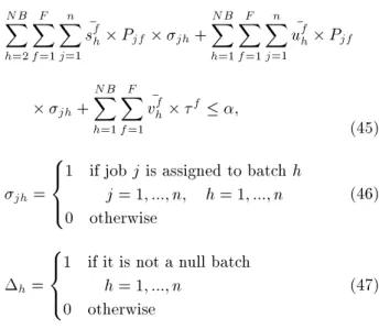
which is obtained from the MP solution, Eq. (32) is objective function of the maximization dual problem subject to Constraints (33)-(40). The Benders cut is deduced from the solution of the DSP at the end of each iteration and it is added to the Master Problem (MP):
MP :
Minimize Z3= ; (41) n
X
h=1
jh= 1; j = 1; :::; n; (42)
h h+1 h = 1; :::; n 1; (43) n
X
j=1
NB X h=2 F X f=1 n X j=1
sfh Pjf jh+ NB X h=1 F X f=1 n X j=1 ufh Pjf
jh+ NB X h=1 F X f=1
vfh f ;
(45) jh= 8 > < > :
1 if job j is assigned to batch h j = 1; :::; n; h = 1; :::; n 0 otherwise (46) h= 8 > < > :
1 if it is not a null batch h = 1; :::; n
0 otherwise
(47)
sfh, ufh, vfh, and wfh are the solutions of DSP to sfh, ufh, vfh, and wfh are considered to have xed values in MP (note that since the SP would never generate the infeasible solution to our problem, feasibility cut is not required to be added to the MP). After solving MP, the lower and upper bounds of the problem are calculated to investigate whether the method should be terminated or continued.
4. Experimental results
This section contains the computational experiments for evaluation of the proposed Benders decomposition method for the mentioned problem. The algorithm is coded in commercial software GAMS and executed on a PC with Intel Core 2 Duo and 2 GB of RAM memory. To the best knowledge of the authors, this paper is a novel research in the scheduling eld; therefore, there is lack of benchmark or competent study on this problem for evaluating the method. Thus random datasets for dierent sizes of the problem are generated for assessing and checking eciency of the method against an adapted B&B presented in [12]. Features of the generated test problems are described in the following; then, the computational experiments are presented.
We generate 10 random data sets of dierent problem sizes with number of jobs ranging from 5 to 200 and number of factories ranging from 2 to 8. All the processing times and transportation times are generated randomly using uniform distribution with parameters [1,99] and [50,200], respectively. Capacity of each transportation vehicle has a uniform distri-bution with parameters [2,20]. Coecient of trans-portation is considered in cases of equal, greater, and smaller than the coecient of make-span using the values 10 and 1000. The optimality gap and maximum number of iterations of the Benders decomposition as stopping criteria of the method are set to 0.01 and
Table 1. Size of instances according to dierent values of number of jobs and factories.
jnj jF j Constraints Variables
5 2 76 88
5 5 133 118
10 2 177 112
10 5 288 170
15 2 334 142
15 5 478 185
20 2 541 172
20 5 763 269
50 2 2851 368
50 5 3538 748
100 2 10701 693
100 5 12003 1374
150 2 23563 1027
150 5 25798 1691
200 2 41401 1383
200 5 42913 1939
40, respectively. In order to show the size alteration through dierent instances, Table 1 is presented, which contains number of constraints and variables that are involved for solving Benders decomposition.
Seeking to evaluate the performance of our ap-proach, dierent experiments are considered in terms of lower and upper bounds, objective function value, computing times, and number of Benders cuts. First, for illustrating the progression of upper- and lower-bound values through iterations, Figure 1 is presented. This gure shows these iterative values for the problem instance with 100 jobs and 5 factories.
It is clear from the gure that deviation of the lower and upper bounds narrows during iterations until the algorithm meets the convergence criteria (the allowed gap between lower and upper bounds) through 19 iterations and, then, it stops.
For investigating computing times and quality of the solution, the method is compared with an adapted B&B algorithm [12] for this problem, which is capable of nding exact solution. Note that the execution times of both methods are limited to 6000 (s) and if the method cannot nd the solution for an instance in that time limit, (-) is put in the relative cell of the table.
The columns O.F and R.T represent objective function values and run times of each method and the column cuts shows the number of cuts generated by Benders method to nd the solution. Vars and Cons are representatives of numbers of variables and
constraints generated by the Benders decomposition method and the Gap value is the relative deviation of the Benders decompositions objective function value from the objective function value of the exact solution of B&B.
Tables 2-4 display the computational results of the mentioned comparison. It is clear that, since B&B achieves the exact solution, the quality of its solution is better than the solution of Benders decomposition but its procedure is too time-consuming in nding the solution. Though, the performance of Benders decomposition can be investigated by means of its
Table 2. Comparison of Benders decomposition performance with branch and bound for = ( = 10 and = 10).
n F Branch and bound Benders decomposition
O.F R.T O.F R.T Cuts Vars Cons GAP
5 2 5940 0.267 6300 1.123 4 64 41 0.060606
5 5 12040 0.424 12540 0.78 4 103 59 0.041528
5 8 18200 0.438 18780 0.646 3 166 93 0.031868
10 2 9410 0.38 9450 1.43 6 201 98 0.004251
10 5 15330 2.658 16720 0.937 4 288 134 0.090672
10 8 20400 6.636 21120 3.421 11 411 206 0.035294
15 2 11700 1.07 11730 1.43 4 334 106 0.002564
15 5 17730 174.65 19130 2.92 8 448 158 0.078962
15 8 22960 275.48 25050 2.346 6 562 204 0.091028
20 2 14120 2.113 14120 2.27 5 571 162 0
20 5 20100 2409.59 20520 5.282 13 823 304 0.020896
20 8 { { 28200 3.876 8 1027 396 {
50 2 29980 10.75 30070 3.21 5 2857 337 0.003002
50 5 35960 4466 37970 10.11 11 3238 499 0.055895
50 8 { { 43830 32.841 25 3811 805 {
100 2 51720 81.688 51720 17.97 6 10923 843 0
100 5 60330 258.59 60550 111.29 15 12003 1374 0.003647
100 8 { { 71600 236.84 24 13275 2041 {
150 2 78130 322.76 77600 28.028 3 24001 1355 0.00683
150 5 { { 85130 2773.39 39 25798 2291 {
150 8 { { 96520 923.54 29 27259 2943 {
200 2 102670 784.1 103500 155.97 5 41407 1312 0.008084 200 5 109640 2510.747 110290 2060.31 26 42913 1939 {
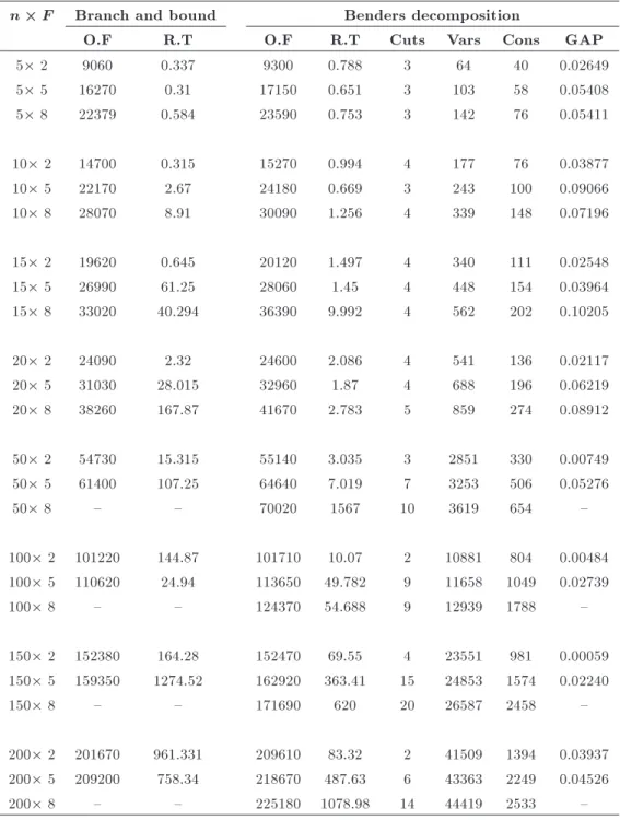
Table 3. Comparison of Benders decomposition performance with branch and bound for < ( = 10 and = 1000).
n F Branch and bound Benders decomposition
O.F R.T O.F R.T Cuts Vars Cons GAP
5 2 9060 0.337 9300 0.788 3 64 40 0.02649
5 5 16270 0.31 17150 0.651 3 103 58 0.05408
5 8 22379 0.584 23590 0.753 3 142 76 0.05411
10 2 14700 0.315 15270 0.994 4 177 76 0.03877
10 5 22170 2.67 24180 0.669 3 243 100 0.09066
10 8 28070 8.91 30090 1.256 4 339 148 0.07196
15 2 19620 0.645 20120 1.497 4 340 111 0.02548
15 5 26990 61.25 28060 1.45 4 448 154 0.03964
15 8 33020 40.294 36390 9.992 4 562 202 0.10205
20 2 24090 2.32 24600 2.086 4 541 136 0.02117
20 5 31030 28.015 32960 1.87 4 688 196 0.06219
20 8 38260 167.87 41670 2.783 5 859 274 0.08912
50 2 54730 15.315 55140 3.035 3 2851 330 0.00749
50 5 61400 107.25 64640 7.019 7 3253 506 0.05276
50 8 { { 70020 1567 10 3619 654 {
100 2 101220 144.87 101710 10.07 2 10881 804 0.00484 100 5 110620 24.94 113650 49.782 9 11658 1049 0.02739
100 8 { { 124370 54.688 9 12939 1788 {
150 2 152380 164.28 152470 69.55 4 23551 981 0.00059 150 5 159350 1274.52 162920 363.41 15 24853 1574 0.02240
150 8 { { 171690 620 20 26587 2458 {
200 2 201670 961.331 209610 83.32 2 41509 1394 0.03937 200 5 209200 758.34 218670 487.63 6 43363 2249 0.04526
200 8 { { 225180 1078.98 14 44419 2533 {
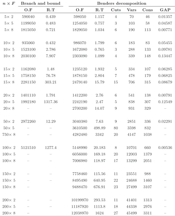
run time and gap. By increasing the size of problem instances, the advantage of Benders decomposition, in terms of computational time, intensies relative to the B&B. For smaller sizes of the instances, it expends larger computational time than B&B. As B&B is an exact solution approach, it is not capable of nding solution for large problem instances in a reasonable time. It is obvious that for larger sizes of the problem, Benders decomposition searches the solution space in bigger number of iterations and, thus, bigger number of cuts are generated for guiding the search procedure.
From the objective function and gap values for the Benders decomposition, it is understood that it can nd near-optimal solution in very smaller time than the B&B.
5. Conclusion
In this paper, we have presented the Benders decom-position to solve a multi-factory scheduling with batch delivery among factories and also to the nal customer. The problem entails minimizing the costs associated with maximum completion time and transportation in
Table 4. Comparison of Benders decomposition performance with branch and bound for > ( = 1000 and = 10).
n F Branch and bound Benders decomposition
O.F R.T O.F R.T Cuts Vars Cons GAP
5 2 590040 0.439 598050 1.157 4 70 46 0.01357
5 5 1199050 0.483 1254050 0.757 3 103 58 0.04587
5 8 1815050 0.721 1829050 1.034 6 190 113 0.00771
10 2 935060 0.432 986070 1.799 6 183 83 0.05455
10 5 1523100 2.786 1672080 0.765 3 288 133 0.09781
10 8 2030100 7.907 2303090 1.099 4 339 148 0.13447
15 2 1162080 1.48 1235120 1.932 5 334 107 0.06285
15 5 1758150 76.78 1878150 2.804 7 478 179 0.06825
15 8 2281150 303.21 2479140 15.79 15 706 315 0.08679
20 2 1401110 1.791 1412200 2.76 6 541 138 0.00791
20 5 1992180 1317.36 2242190 2.47 5 838 307 0.12549
20 8 { { 2700200 14.07 9 931 329 {
50 2 2972260 12.29 3040380 7.63 9 2851 336 0.02291
50 5 { { 3610500 498.89 80 3598 832 {
750 8 { { 4282480 3342 20 4147 1038 {
100 2 5121510 1277.4 5148990 20.183 8 10701 660 0.00536
100 5 { { 6056000 169.18 20 12003 1379 {
100 8 { { 7006980 118.97 17 13299 2051 {
150 2 { { 7758460 115.56 11 23551 988 {
150 5 { { 8495490 640.95 22 24688 1460 {
150 8 { 9488470 676.91 23 27499 3107 {
200 2 { { 10199970 293.53 11 41401 1313 {
200 5 { { 11187920 1113.8 18 44338 2976 {
200 8 { 12038970 1624 27 45499 3311 {
the system and at the end of the system. The main contribution of this paper is Benders reformulation of the problem, which facilitates the solution approach by decomposing the hard problem to two simpler prob-lems. The objective function of the master problem can also be considered as the lower bound of the original problem.
Numerical experiments were conducted to eval-uate the eciency of the proposed method tackling a large-scale real-world problem. The comparison of this method with the exact solution approach, adapted B&B method, presented in [12] is performed. The experimental results conrm the superior performance
of our presented method in terms of the run time to the B&B algorithm, especially for a larger number of problem instances. It is clear that for larger sizes, the B&B cannot nd the solution in reasonable time; but, Benders decomposition is capable of nding near-optimal solution in the considered time.
For future research, we are seeking for ways to accelerate the Benders decomposition algorithm, such as developing a method to generate a set of cuts at each iteration, for this problem. In addition, some more research can be done with dierent assumptions of this problem, like unlimited number of vehicles, unlimited buers, etc.
References
1. Moon, C., Seo, Y., Yun, Y. and Gen, M. \Adaptive genetic algorithm for advanced planning in manufac-turing supply chain", J. Intell. Manuf., 17, pp. 509-522 (2006).
2. Moon, C. and Seo, Y. \Evolutionary algorithm for advanced process planning and scheduling in a multi-plant", Comput. Ind. Eng., 48, pp. 311-325 (2005). 3. Karatza, H.D. \Job scheduling in heterogeneous
dis-tributed systems", Journal of Systems and Software, 56(3), pp. 203-212 (2001).
4. Moon, C., Kim, J. and Hur, S. \Integrated process planning and scheduling with minimizing total tar-diness in multi-plants supply chain", Computers & Industrial Engineering, 43(1-2), pp. 331-349 (2002). 5. Jia, H.Z., Nee, A.Y.C., Fuh, J.Y.H. and Zhang, Y.F.
\A modied genetic algorithm for distributed schedul-ing problems", Journal of Intelligent Manufacturschedul-ing, 14(3-4), pp. 351-362 (2003).
6. Chan, F.T.S., Chung, S.H. and Chan, P.L.Y. \An adaptive genetic algorithm with dominated genes for distributed scheduling problems", Expert Systems with Applications, 29(2), pp. 364-371 (2005).
7. Chan, F.T.S., Chung, S.H. and Chan, P.L.Y. \Appli-cation of genetic algorithms with dominant genes in a distributed scheduling problem in exible manufac-turing systems", International Journal of Production Research, 44(3), pp. 523-543 (2006).
8. Chung, S.H., Lau, H.C.W., Choy, K.L., Ho, G.T.S. and Tse, Y.K. \Application of genetic approach for advanced planning in multi-factory environment", In-ternational Journal of Production Economics, 127(2), pp. 300-308 (2010).
9. Sun, X.T., Chung, S.H. and Chan, F.T.S. \Integrated scheduling of a multi-product multi-factory manufac-turing system with maritime transport limits", Trans-portation Research Part E, 79, pp. 110-127 (2015). 10. H'Mida, F. and Lopez, P. \Multi-site scheduling under
production and transportation constraints", Interna-tional Journal of Computer Integrated Manufacturing, 26(3), pp. 252-266 (2013).
11. Huang, J.-Y. and Yao, M.-J. \On the optimal lot-sizing and scheduling problem in serial-type supply chain system using a time-varying lot-sizing policy", International Journal of Production Research, 51(3), pp. 735-750 (2013).
12. Karimi, N. and Davoudpour, H. \A branch and bound method for solving multi-factory supply chain scheduling with batch delivery", Expert Systems with Applications, 42, pp. 238-245 (2015).
13. Potts, C.N. \Technical notes analysis of a heuristic for one machine", Operation Research, 28(6), pp. 1436-1441 (1980).
14. Herrmann, J.W. and Lee, C.-Y. \On scheduling to minimize earliness-tardiness and batch delivery costs with a common due date", European Journal of Oper-ational Research, 70, pp. 272-288 (1993).
15. Cheng, T.C.E., Gordon, V.S. and Kovalyov, M.Y. \Single machine scheduling with batch deliveries", European Journal of Operational Research, 94(2), pp. 277-283 (1996).
16. Hall, N.G. and Potts, C.N. \Supply chain scheduling: Batching and delivery", Operations Research, 51(4), pp. 566-584.
17. Mahdavi-Mazdeh, M., Shashaani, S., Ashouri, A. and Hindi, K.S. \Single-machine batch scheduling minimiz-ing weighted ow times and delivery costs", Applied Mathematical Modelling, 35(1), pp. 563-570 (2011). 18. Mahdavi-Mazdeh, M., Sarhadi, M. and Hindi, K.S.
\A branch-and-bound algorithm for single-machine scheduling with batch delivery minimizing ow times and delivery costs", European Journal of Operational Research, 183, pp. 74-86 (2007).
19. Mahdavi-Mazdeh, M., Sarhadi, M. and Hindi, K.S. \A branch-and-bound algorithm for single-machine scheduling with batch delivery and job release times", Computers & Operations Research, 35, pp. 1099-1111 (2008).
20. Rasti-barzoki, M. and Hejazi, S.R. \Minimizing the weighted number of tardy jobs with due date assign-ment and capacity-constrained deliveries for multiple customers in supply chains", European Journal of Operational Research, 228(2), pp. 345-357 (2013). 21. Benders, J. \Partitioning procedures for solving mixed
variables programming problems", Numerische Math-ematik, 4, pp. 238-252 (1962).
22. Hooker, J.N. \Planning and scheduling to minimize tardiness", In Lecture Notes in Computer Science. Principles and Practice of Constraint Programming, 3709, pp. 314-327 (2005).
23. Hooker, J.N. \An integrated method for planning and scheduling to minimize tardiness", Constraints, 11, pp. 139-157 (2006).
24. Hooker, J.N. \Planning and scheduling by logic-based benders decomposition planning and scheduling by logic-based benders decomposition", Operations Re-search, 55(3), 588-602 (2007).
25. Rinnooy Kan, A.H. G., Machine Scheduling Problems: Classication, Complexity and Computations, Marti-nus Nijho, The Hague, Neth (1976).
Biographies
Neda Karimi received her PhD degree in Industrial Engineering in 2016. Her research is mainly focused on scheduling, supply chain, and mathematical modeling. Hamid Davoudpour has been a Faculty Member at Amikabir University, Tehran, Iran, since 1978.
He is currently Associate Professor in the Faculty of Industrial and Systems Engineering and Manage-ment.
His research interests include production planning and scheduling, and locations and allocation problems.
He is Chief Editor of International Journal of Modern Science and Technology. He has published 12 books and more than 150 papers in international journals and presented many others at national and international conferences.