HYDROGEOMORPHIC CONTROLS ON BENTHIC LIGHT AVAILABILITY IN RIVERS
Jason Paul Julian
A dissertation submitted to the faculty of the University of North Carolina at Chapel Hill in partial fulfillment of the requirements for the degree of Doctor of Philosophy in the Department of Geography.
Chapel Hill 2007
ABSTRACT
Julian, J.P., Ph.D., University of North Carolina at Chapel Hill, August 2007. Hydrogeomorphic Controls on Light Availability in Rivers
(Under the direction of Martin W. Doyle)
Light is vital to the dynamics of aquatic ecosystems. It drives photosynthesis and photochemical reactions, affects thermal structure, and influences the behavior of aquatic biota. While the influence of hydrology and geomorphology on other ecosystem-limiting factors have been well studied (e.g., habitat, nutrient cycling), the more fundamental limitation of light availability has received much less attention. In this thesis, I analyzed and quantified the hydrogeomorphic controls on benthic (or riverbed) light availability using a combination of meta-analyses, field studies, laboratory studies, and model simulations. I developed a benthic light availability model (BLAM) that predicts
photosynthetically active radiation (PAR) at the riverbed (Ebed) by calculating the amount
of above-canopy PAR that is attenuated by all five hydrogeomorphic controls:
topography, riparian vegetation, channel geometry, optical water quality, and hydrologic regime. This model was used to assess and characterize broad spatial patterns of Ebed and
temporal variations associated with variable flow conditions for a wide range of rivers. BLAM was also used to assess the effects of riparian deforestation and degraded optical water quality associated with agriculturalization on Ebed. BLAM is the first model to
quantify Ebed using all five hydrogeomorphic controls, and thus provides a new tool that
availability targets in water resource management. BLAM also provides a framework for future models to characterize spatiotemporal variations of ultraviolet and infrared
ACKNOWLEDGEMENTS
This research was primarily funded by the National Research Initiative of the USDA Cooperative State Research, Education, and Extension Service (CSREES grant # 2004-35102-14793). Additional support was provided by NSF grant DEB-0321559US, U.S. Fish and Wildlife Service, and Restoration Systems, LLC. Special thanks to Bill Ginsler and the town of Big Spring, WI for site access. Helen Sarakinos of the
Wisconsin River Alliance and Marty Melchior and Andy Selle of Inter-fluve, Inc. were also instrumental in research logistics.
I am grateful for the assistance provided by numerous faculty, staff, and students from the Departments of Geography, Environmental Science & Engineering, and
PREFACE
Let there be light.
God Genesis 1:3
You cannot step twice into the same river; for other waters are continually flowing in.
Heraclitus
I keep the subject of my inquiry constantly before me, and wait till the first dawning opens gradually, by little and little, into a full and clear light.
TABLE OF CONTENTS
LIST OF TABLES ………. xiii
LIST OF FIGURES ……… xiv
LIST OF SYMBOLS AND ABBREVIATIONS ……….…….. xvi
CHAPTER I. INTRODUCTION ...………... 1
FLUVIAL ECOSYSTEMS AND HYDROGEOMORPHIC CONTROLS …….. 1
ROLE OF LIGHT ……….. 2
PURPOSES AND METHODS ……….. 2
STRUCTURE OF DISSERTATION ……… 3
REFERENCES ……….. 6
CHAPTER II. OPTICAL WATER QUALITY IN RIVERS ………... 7
INTRODUCTION ………. 7
COMPONENTS AND CONTROLS OF OPTICAL WATER QUALITY …….. 8
Pure Water ………... 10
Chromophoric Dissolved Organic Matter ……… 10
Suspended Sediment ……… 12
Particulate Organic Matter ………13
Phytoplankton ……….. 14
Synopsis ………... 16
Deep River ……….……….. 17
Big Spring Creek ……….………. 18
Baraboo River ……….. 19
Wisconsin River ………... 19
METHODS ……….. 20
Sample Collection ……… 20
Hydrology ……… 21
Water Chemistry ……….. 21
Optical Measurements ………. 22
Partitioning the Light Attenuation Coefficient ……… 25
Optical Water Quality Budget ………. 26
Synoptic Optical Water Quality Datasets ……… 27
RESULTS ……… 27
Optical Water Quality Comparisons ……… 27
Temporal Trends: Deep River and Big Spring Creek ……….. 29
Spatial Trends: Baraboo River and Wisconsin River ………... 33
Optical Water Quality Budget of Baraboo River ………..… 35
DISCUSSION ………. 36
Riverine Optical Water Quality ………... 36
OWQ across the Hydrograph ………... 39
OWQ along the River Continuum ……….…... 41
CONCLUSIONS ………. 46
CHAPTER III. EMPIRICAL MODELING OF LIGHT AVAILABILITY
IN RIVERS ……….. 67
INTRODUCTION ………... 67
METHODS ……….. 70
Model Development ………. 70
Study Sites ………... 73
Data Collection and Model Inputs ………... 75
Data Analysis ………... 77
Model Assumptions and Limitations ………... 80
RESULTS ……… 81
Controlling Parameters ……… 81
Temporal Light Availability ……… 83
Spatial Light Availability ………. 84
Comparisons between Modeled and Actual Benthic PAR ……….. 86
DISCUSSION ……….…. 87
Controls on Riverine Benthic Light Availability ……….… 87
Small vs. Large Rivers ………. 89
Applications of BLAM ……… 91
CONCLUSIONS ………. 93
REFERENCES ……… 95
CHAPTER IV. LIGHT ALONG THE RIVER CONTINUUM ………... 114
INTRODUCTION ………. 114
METHODS ……… 118
Modeling Basin-Scale Benthic PAR ……….. 118
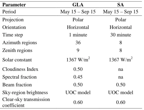
Model Parameters ………... 119
Model Assumptions ……….... 123
Model Simulations ……….…. 123
Primary Productivity ………... 125
RESULTS ……….. 125
Empirical Parameters from Synoptic Survey ………. 125
Modeled Parameters from GIS Analysis ……….………... 126
Benthic PAR along Baraboo River ……….… 128
Benthic PAR under Model Simulations …….………. 129
DISCUSSION ……… 132
Basin-Scale Benthic Light Availability ………. 132
Effect of Agriculturalization on Benthic Light Availability ………….. 134
Other Disturbances on Benthic Light Availability ….……… 136
Implications of Altered Riverine Light Regimes ………... 138
CONCLUSIONS ………... 139
REFERENCES ……….. 140
CHAPTER V. CONCLUSIONS ……….. 155
RESEARCH OBJECTIVES AND THESIS STRUCTURE ………. 155
SPATIAL AND TEMPORAL TRENDS IN BENTHIC LIGHT AVAILABILITY ………... 157
LIST OF TABLES
2.1 Temporal sampling of OWQ at BSC and DR ……….. 53
2.2 Partitioning of the light attenuation coefficient ………... 53
2.3 Discharge and water chemistry of study sites ……….. 54
2.4 Baseflow OWQ of study sites ……….. 54
2.5 Partitioned OWQ for Deep River and Big Spring Creek ………. 55
2.6 Predicted vs. actual tributary effects on OWQ in Baraboo River ……… 55
3.1 GLA user-defined parameters ………..……… 99
3.2 Turbidity sampling at Big Spring Creek and Deep River …..……….. 99
3.3 BLAM input parameters for Big Spring Creek and Deep River ………... 100
3.4 Predicted vs. actual benthic PAR in Big Spring Creek, WI ………….……….. 100
4.1 Gap Light Analyzer and Solar Analyst user-defined parameters …..…………. 145
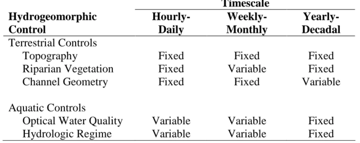
5.1 Effective timescales for the hydrogeomorphic controls on benthic light availability ………. 165
LIST OF FIGURES
2.1 Optical water quality study sites ………...….. 56
2.2 Heuristic diagram of the four-configuration spectrophotometer scan ……...…. 57
2.3 Representative spectrophotometer scans of the four study sites during baseflow ………...… 58
2.4 Light attenuation coefficient vs. turbidity for the four study sites …………... 59
2.5 Discharge and turbidity record for Deep River and Big Spring Creek …...…… 60
2.6 Temporal OWQ of Big Spring Creek and Deep River ……… 61
2.7 Contributions of OWQ components to the total light attenuation coefficient at Deep River and Big Spring Creek during baseflow ………...…. 62
2.8 Longitudinal profile of water chemistry, elevation, and optical water quality along Wisconsin River ……… 63
2.9 Longitudinal profile of water chemistry, elevation, and optical water quality along Baraboo River ………...… 64
2.10 Optical water quality budget for Baraboo River ………. 65
2.11 OWQ along the river continuum ………. 66
3.1 Light availability in rivers ………...… 101
3.2 Hemispherical canopy photos of transects at Big Spring Creek and Deep River ……….. 102
3.3 Big Spring Creek and Deep River study reaches ……….…. 103
3.4 Longitudinal profile of Big Spring Creek and Deep River ……… 104
3.5 Temporal distribution of daily above-canopy PAR, discharge, and benthic PAR at Big Spring Creek and Deep River ……… 105
3.6 Diffuse attenuation coefficient vs. turbidity for Big Spring Creek and Deep River ……….. 106
3.8 Magnitude-frequency distributions of benthic light availability at
Big Spring Creek and Deep River ……….… 108 3.9 Longitudinal distribution of above-canopy PAR, below-canopy PAR, and
benthic PAR during baseflow at Big Spring Creek and Deep River …………. 109 3.10 Spatial comparisons of longitudinal benthic PAR with shading coefficient
and water depth for Big Spring Creek and Deep River ……….… 110 3.11 Effect of channel orientation on shading coefficients ……… 111 3.12 Predicted benthic PAR vs. actual benthic PAR at Big Spring Creek ………… 112 3.13 Benthic light availability along the river continuum of an idealized
10th-order river with a continuous forested riparian corridor ………... 113 4.1 Conceptual profile of benthic light availability along the continuum
of a forested river ………... 146
4.2 Baraboo River Basin ……….. 147
4.3 Schematic of the GIS framework to model basin-scale
benthic light availability ……… 148 4.4 Vegetation shading coefficient curves based on channel width
and orientation ………... 149 4.5 Downstream variation in width and depth along Baraboo River ………... 150 4.6 Downstream variation in the diffuse attenuation coefficient for
LIST OF SYMBOLS AND ABBREVIATIONS
α Empirical coefficient for relating y to Q a Total absorption coefficient (m-1)
ad Absorption coefficient of dissolved constituents (m-1)
ap Absorption coefficient of particulates (m-1)
aw Absorption coefficient of pure water (m-1)
a440 Absorption coefficient at 440 nm (m-1)
AMSL Above Mean Sea Level ANOVA ANalysis Of VAriance model
β Empirical coefficient for relating Kd to Q
b Total scattering coefficient (m-1)
bd Scattering coefficient of dissolved constituents (m-1)
bp Scattering coefficient of particulates (m-1)
bw Scattering coefficient of pure water (m-1)
bPOM Scattering coefficient of particulate organic matter (m-1)
BLAM Benthic Light Availability Model BSC Big Spring Creek
BR Baraboo River
c Total light (beam) attenuation coefficient (m-1)
cd Light attenuation coefficient of dissolved constituents (m-1)
cp Light attenuation coefficient of particulates (m-1)
cw Light attenuation coefficient of pure water (m-1)
CDOM Chromophoric dissolved organic matter D Absorbance (log10Ф0/Ф)
D Kolmogorov-Smirnov test statistic for a normal distribution DEM Digital Elevation Model
DOC Dissolved organic carbon (mg/L) DR Deep River
E0 Below-water surface PAR (mol/m2/day)
Ebed Benthic PAR (mol/m2/day)
Ecan Above-canopy PAR (mol/m2/day)
Es Above-water surface PAR (mol/m2/day)
F Filtered water sample
GLA Gap Light Analyzer software IR Infrared solar radiation K bPOM/aPOM
Kd Diffuse attenuation coefficient for downward PAR (m-1)
LAI Leaf Area Index
LCM Land-cover Classification Map NTU Nephelometric turbidity units OWQ Optical water quality
Ф0 Incident radiant flux (mol/s) Ф Transmitted radiant flux (mol/s)
POM Particulate organic matter (mg/L)
PPFD Photosynthetic photon flux density (µmol/m2/s) Q Discharge or volume of water per time (m3/s) Qpeak Maximum discharge during a flood
Qds Discharge of river just downstream of a tributary (m3/s)
Qtrib Discharge of tributary just before confluence with mainstem (m3/s)
Qus Discharge of river just upwnstream of a tributary (m3/s)
r Reflection coefficient r2 Coefficient of determination RCC River Continuum Concept s Shading coefficient
st Topographic shading coefficient
sv Vegetation shading coefficient
SCH Standard cell holder; used to obtain a SS Suspended Sediment (mg/L)
Tn Turbidity (NTU)
TCH Turbidity cell holder; used to obtain c TSS Total suspended solids (mg/L)
UF Unfiltered water sample UV Ultraviolet solar radiation
υ Empirical exponent for relating y to Q VIS Visible solar radiation
WR Wisconsin River
Χ Apparent absorption coefficient (m-1) y Water depth (m)
yBD Black disk visibility distance (m)
CHAPTER I. INTRODUCTION
“Meeting human water needs and sustaining the services that aquatic ecosystems provide remain one of the greatest challenges of the 21st century.”
- Palmer & Bernhardt 2006 FLUVIAL ECOSYSTEMS AND HYDROGEOMORPHIC CONTROLS
Fluvial ecosystems are shaped by the hydrologic and geomorphic template (Hynes 1970, Poff and Ward 1990). This hydrogeomorphic template includes basin topography, land cover, channel geometry, sediment size, and the quantity and quality of water. The variability of these controls, together with their interdependent relationships, create fluvial ecosystems that are dynamic over both space and time. Some researchers have gone so far to say that the multiplicity and variability of hydrogeomorphic controls prevent generalizations on ecosystem dynamics (Phillips 2007). Yet, scientists are expected to decipher these general trends and develop predictive models that can be used to preserve and rehabilitate anthropogenic damaged aquatic ecosystems (Palmer and Bernhardt 2006).
An emerging theme in fluvial ecology is to predict spatiotemporal trends of ecosystem variables using empirical correlations to hydrogeomorphic controls. Examples include correlating organic matter and nutrient transport to discharge (Doyle et al. 2005), fish distribution to suspended sediment concentration (Burcher et al. 2007),
coupling of hydrogeomorphology and fluvial ecology has led to several key contributions in the field (e.g., nutrient spiraling concept; Newbold et al. 1982), we have only begun to understand how spatiotemporal variations in hydrogeomorphic controls structure fluvial ecosystems.
ROLE OF LIGHT
The influence of hydrology and geomorphology on ecosystem-limiting factors has been well studied, particularly habitat availability and nutrient cycling (e.g., Doyle and Stanley 2006, Strayer et al. 2006); however, the more fundamental limitation of light availability has received much less attention. Light is the primary energy source of rivers, driving photosynthesis and photochemical reactions, dictating thermal
fluctuations, and influencing the behavior of aquatic biota (Wetzel 2001, p. 49). Davies-Colley et al. (2003) argues that the neglect of riverine light studies can be attributed to (i) light not being widely accepted as a limiting resource in riverine ecosystems, (ii)
boundary conditions (banks, riparian vegetation) making ambient light measurements challenging, and (iii) the optical water quality of rivers being highly variable and difficult to characterize. The little information that is available on light in rivers is derived mostly from New Zealand rivers under predominantly baseflow conditions, leaving substantial limitations in our understanding of the temporal and spatial availability of light in rivers.
PURPOSES AND METHODS
and temporal variability, and develop a model for predicting benthic light availability using readily available or easily collected data. The fundamental questions addressed within this thesis were:
1. What are the dominant controls of benthic light availability in rivers?
2. Do spatial and temporal variations in benthic light availability follow general trends?
3. How is benthic light availability affected by anthropogenic disturbances? The above questions were answered using a combination of meta-analyses, field studies, laboratory studies, and model simulations. Field studies were conducted on four rivers: Big Spring Creek – a 2nd-order spring-fed stream in central Wisconsin; Deep River – a 6th-order river in central North Carolina; Baraboo River – a 6th-order river in central Wisconsin , and Wisconsin River – a 7th-order river that empties into the Mississippi River. Laboratory studies were performed on water samples collected from these four rivers.
STRUCTURE OF DISSERTATION Papers Presented in Chapters
This thesis is written in the form of 3 chapters, all of which are independent manuscripts for journal submission, followed by a conclusion. There is some repetition of introductory material, but this was done so that the manuscripts could stand alone.
new method for partitioning the light attenuation coefficient into its constituent fractions. Third, it compares the baseflow optical water quality of four rivers with vastly different physical characteristics. Fourth, it analyzes spatial and temporal distributions of optical water quality for the four rivers. Fifth, it calculates an optical water quality budget for one of the rivers based on tributary inputs. Finally, this chapter compares spatial trends (i.e., along the river continuum from headwaters to mouth) of optical water quality between American and New Zealand rivers, paying particular attention to the magnitude and shape of the longitudinal distributions.
Chapter 3 introduces the reach-scale Benthic Light Availability Model (BLAM), which calculates the amount of daily photosynthetically active radiation (PAR) that reaches the riverbed (Ebed; in mol/m2/day). First, it describes model development,
detailing how each hydrogeomorphic control influences benthic light availability. Second, it presents model output for two rivers with vastly different physical
characteristics: Big Spring Creek and Deep River. Third, it assesses model accuracy by comparing modeled Ebed to in situ measurements of Ebed. Finally, it identifies the
dominant controls on benthic light availability in rivers by comparing correlations between the hydrogeomorphic controls and Ebed.
Chapter 4 demonstrates how BLAM can be applied to the basin-scale by using a GIS framework. This GIS-based model was used to calculate Ebed along the 187-km
mainstem of the Baraboo River, Wisconsin . This chapter also uses three model
simulations to demonstrate how various levels of agricultural land conversion affect Ebed
Manuscript Details
CHAPTER 2: Julian, J.P., M.W. Doyle, S.M. Powers, E.H. Stanley, and J.A. Riggsbee. Optical water quality in rivers. Water Resources Research.
CHAPTER 3: Julian, J.P., M.W. Doyle, and E.H. Stanley. Empirical modeling of light availability in rivers. Journal of Geophysical Research - Biogeosciences. CHAPTER 4: Julian, J.P., M.W. Doyle, and E.H. Stanley. Light along the river
REFERENCES
Burcher, C. L., H. M. Valett, and E. F. Benfield. 2007. The land-cover cascade: Relationships coupling land and water. Ecology 88:228-242.
Davies-Colley, R. J., W. N. Vant, and D. G. Smith. 2003. Colour and Clarity of Natural Waters. Ellis Horwood, New York.
Doyle, M. W., and E. H. Stanley. 2006. Exploring potential spatial-temporal links between fluvial geomorphology and nutrient-periphyton dynamics in streams using simulation models. Annals of the Association of American Geographers 96:687-698.
Doyle, M. W., E. H. Stanley, D. L. Strayer, R. B. Jacobson, and J. C. Schmidt. 2005. Effective discharge analysis of ecological processes in streams. Water Resources Research 41:1-16.
Gangloff, M. M., and J. W. Feminella. 2007. Stream channel geomorphology influences mussel abundance in southern Appalachian streams, USA. Freshwater Biology 52:64-74.
Hynes, H. B. N. 1970. The Ecology of Running Waters. University of Toronto Press, Toronto.
Newbold, J. D., P. J. Mulholland, J. W. Elwood, and R. V. O'Neill. 1982. Organic carbon spiralling in stream ecosystems. Oikos 38:266-272.
Palmer, M. A., and E. S. Bernhardt. 2006. Hydroecology and river restoration: Ripe for research and synthesis. Water Resources Research 42:W03S07,
doi:10.1029/2005WR004354.
Phillips, J. D. 2007. The perfect landscape. Geomorphology 84:159-169.
Poff, N. L., and J. V. Ward. 1990. Physical habitat template of lotic systems: Recovery in the context of historical pattern of spatiotemporal heterogeneity. Environmental Management 14:629-645.
Strayer, D. L., H. M. Malcolm, R. E. Bell, S. M. Carbotte, and F. O. Nitsche. 2006. Using geophysical information to define benthic habitats in a large river. Freshwater Biology 51:25-38.
CHAPTER II. OPTICAL WATER QUALITY IN RIVERS
1. INTRODUCTION
Optical water quality (OWQ) is “the extent to which the suitability of water for its functional role in the biosphere or the human environment is determined by its optical properties” (Kirk 1988). Accordingly, OWQ governs the behavior of photons in aquatic ecosystems and determines underwater light quantity (number of photons) and quality (wavelength). It therefore influences primary productivity, water temperature, faunal movements, photo-degradation of organic matter, and numerous other photo-assisted biogeochemical reactions (Wetzel 2001). Changes in OWQ can indicate important environmental trends such as eutrophication, sedimentation, or general water quality degradation. Additionally, OWQ is a key component of aesthetics, recreation, and management of water resources. Thus, OWQ is a master variable that both reflects prevailing environmental conditions and dictates multiple aspects of structure and function in these ecosystems.
The significance of light has long been recognized in oceans, estuaries, and lakes, but has mostly been dealt with in a descriptive, qualitative fashion in rivers. Of the body of work that exists on rivers, most address only individual influences such as light
riverine OWQ. The lack of data persists despite the central role ascribed to light availability in fluvial ecology models such as the River Continuum Concept (RCC; Vannote et al. 1980). Nonetheless, the eclectic nature of OWQ and the ease of field measurement has resulted in its adoption as a water quality standard in some countries (Davies-Colley et al. 2003).
The goal of this paper is to provide a comprehensive overview of the controls and the spatial and temporal dynamics of riverine OWQ, and place this understanding in the context of prevailing fluvial ecosystem theory. First, the constituents influencing OWQ are reviewed, focusing on the spatiotemporal trends in rivers. Second, a new method is developed for partitioning the light attenuation coefficient into its constituent fractions. Third, we compare baseflow OWQ between four rivers with vastly different physical characteristics to illustrate its inter-site variability. Fourth, we analyze the spatial and temporal distributions of OWQ for the four rivers. Fifth, we quantify an OWQ budget for one of the rivers, including tributary inputs. Finally, available data are synthesized to identify general spatial trends robust across broad geographic areas.
scattered by an infinitesimally thin layer of aquatic medium. Together, a and b establish the light (beam) attenuation coefficient (c), the fraction of radiant flux that is lost over the infinitesimally thin layer of aquatic medium, in m-1:
c = a + b (2.1)
Accordingly, c is low for rivers that are optically clear, and high for turbid rivers. The amount of radiant flux at depth (Ф) in the aquatic medium is derived using c in the Beer-Lambert law:
Ф = Ф0*e-cr (2.2)
where Ф0 is incident radiant flux in mol/s (1 mol = 6.02 x 10²³ photons), and r is the
pathlength in m. In rivers, the amount of light at depth is ultimately dictated by the diffuse attenuation coefficient (Kd), which accounts for solar zenith angle, the ratio of
diffuse to direct solar radiation, and diffuse light within the water column. Kd and c are
directly proportional (Kirk 1994), and thus trends in Kd follow those of c. In examining
the OWQ of rivers, however, only the values of a, b, and c are of interest because they are the inherent optical properties (i.e., not dependent on the solar radiation field) of the aquatic medium.
Any component of the water column can absorb and scatter light, but there are only five that significantly attenuate light in rivers: water (w), chromophoric dissolved organic matter (CDOM), suspended sediment (SS), particulate organic matter (POM), and phytoplankton (PHYTO) (Davies-Colley et al. 2003). Because light attenuation is an additive process (Kirk 1994), the sum of light attenuation by each one of these
components sets the OWQ of a river such that:
c = cw + cd + cp (2.4)
where cd is the attenuation coefficient of the dissolved constituents (cCDOM) and cp is the
attenuation coefficient of the particulate constituents (cSS + cPOM + cPHYTO). We now
briefly review the drivers of spatial and temporal variability in each of these attenuation coefficients based on previous literature.
2.1. Pure Water
Water molecules scatter and absorb light; however, the amount of scattering by water in rivers is negligible relative to the total light attenuation by all five components (Davies-Colley et al. 2003). The spectral absorption by water follows a parabolic trend where absorption is high for short (ultraviolet, UV) and long wavelengths (infrared, IR), and low for medium wavelengths (visible, VIS). The light attenuation coefficient of pure water (cw) for photosynthetically active radiation (PAR: 400 – 700 nm) is 0.150 m-1, with
0.148 and 0.002 m-1 being attributed to the absorption coefficient of pure water (aw) and
the scattering coefficient of pure water (bw), respectively (Buiteveld et al. 1994). Because
of their very low light attenuation coefficient, water molecules are only a significant contributor to total light attenuation in the clearest rivers (e.g., undisturbed, spring-fed headwater streams), where there is very little CDOM, SS, POM, or PHYTO.
2.2. Chromophoric Dissolved Organic Matter (CDOM)
molecules, scattering by CDOM in rivers is negligible. CDOM originates mainly from the decomposition of plant tissue into dissolved humic substances that contain
chromophores, the molecular components that absorb light. CDOM is not a commonly analyzed constituent in river studies, but given that CDOM concentrations correlate well with dissolved organic carbon (DOC) concentrations (Wetzel 2001), we rely on the spatial and temporal trends of DOC to illustrate the spatiotemporal trends of CDOM. Most of the DOC present in rivers is delivered by terrestrial groundwater inputs, but can also be derived from canopy throughfall, exudates of aquatic vegetation, in-channel detritus leaching, and animal excretions (Webster et al. 1995). Terrestrially derived DOM has higher concentrations of CDOM compared to in-stream sources (Wetzel 2001). High DOC concentrations are predominantly found in rivers surrounded by wet, sandy soils (Wetzel 2001) and rivers that drain wetland dominated basins (Aitkenhead and McDowell 2000). Conversely, rivers fed by lakes/reservoirs tend to have low DOC concentrations due to the long water residence times allowing greater processing (i.e., removal) of DOC (Larson et al. 2007).
Temporally, DOC concentrations tend to be higher during warmer and wetter periods, and especially high following storms that flush out CDOM from the drainage basin (Walling and Webb 1992, Webster et al. 1995); however, there are exceptions (e.g., Meyer 1986). Rivers that drain wetlands usually experience elevated DOC
The absorption coefficient at 440 nm (a440) is a widely-used index for the
concentration of CDOM (Kirk 1994). Values of a440 for rivers have been observed to be
as low as 0.16 (Ybbs River, Austria) and as high as 12.44 (Carrao River, Venezuela) (Kirk 1994). During baseflow conditions, CDOM is usually the main contributor to light absorption in rivers (Davies-Colley et al. 2003).
2.3. Suspended Sediment
Suspended sediment (SS), also referred to as non-volatile suspended solids (NVSS), is the mineral portion of the total suspended solids (TSS) in rivers. These mineral particulates scatter light strongly, with the magnitude of scattering being dependent on particle size, shape, and composition (Davies-Colley and Smith 2001). Absorbance by mineral particulates is minimal, but there are exceptions when certain compounds are present (e.g., iron oxides; Babin and Stramski 2004). The SS in a river originates from a range of sources within its drainage basin, most from in-channel erosion, surface runoff, and tributary inputs (Walling and Webb 1992). Because fluvial sediment is usually source-limited, SS concentrations largely depend on the drainage basin’s geology, climate regime, topographic relief, level of glaciation, vegetative cover, impoundment distribution, and land-use (Milliman and Meade 1983, Syvitski et al. 2000).
al. 1952). Seasonal trends in SS occur in drainage basins with large ice/snow
accumulations, but for most rivers, temporal distributions of SS are largely dictated by Q (Syvitski et al. 2000). Spatially, SS should decrease in the downstream direction because overland sediment runoff decreases and the contribution of sediment-free groundwater to total Q increases (Leopold and Maddock 1953). However, land-use disturbances such as deforestation, cultivation, and urbanization have caused SS to increase in the downstream direction for most rivers due to increased source inputs (Walling and Webb 1992). Because of their low settling velocity, high attenuation cross-sections (attenuation per unit mass), and prevalence in most rivers, clays and fine silts (0.2 – 8 µm) tend to dominate the overall light attenuation in rivers (Davies-Colley et al. 2003).
2.4. Particulate Organic Matter
Particulate organic matter (POM), also referred to as volatile suspended solids (VSS), is the organic portion of TSS in rivers. POM is effective at both absorbing and scattering light. Its spectral signature is similar to CDOM, where absorption decreases with increasing wavelength. Like SS, the magnitude of scattering by POM is dependent on particle size, shape, and composition (Davies-Colley and Smith 2001). POM
POM has greater seasonality; however, seasonal trends are extremely diverse due to variations in catchment vegetation and hydrologic regime (Webster et al. 1995, Golladay 1997).
Spatial trends in POM are largely controlled by the type and areal coverage of surrounding terrestrial vegetation. Rivers located in forested catchments have relatively high POM concentrations, and those with dense riparian vegetation have particularly high POM concentrations (Golladay 1997). Lower-gradient rivers usually have higher POM concentrations because of their greater connectivity with a broader floodplain that is inundated more frequently (Golladay 1997, Wetzel 2001). Webster, et al. (1995) found that POM concentrations increased slightly in the downstream direction; however, most studies have not found significant longitudinal trends of POM, most likely due to local variations in sources and sinks, dependency on hydrologic regime, and improper sampling strategies (Walling and Webb 1992, Golladay 1997). Next to SS, POM is usually the second most effective OWQ constituent at attenuating light in rivers (Davies-Colley et al. 2003).
2.5. Phytoplankton
colonies (Kirk 1994). The spectral signature of PHYTO is similar to that of POM, but with two distinct absorption peaks at approximately 440 and 675 nm. Potamoplankton (i.e., river phytoplankton) originate from detached benthic populations and inflows from lake/wetland surface waters (Wetzel 2001). While studies have shown the abundance of potamoplankton to be correlated to light (Koch et al. 2004), nutrients (Basu and Pick 1996), temperature (Stevenson and White 1995), and grazing pressure (Caraco et al. 1997), the ubiquitous control on potamoplankton is hydraulic residence time (Soballe and Kimmel 1987, Reynolds 2000, Ameziane et al. 2003, Hilton et al. 2006). Due to the rapid mixing that occurs in rivers, the generation rate of potamoplankton must be faster than their downstream displacement rate for large populations to develop (Reynolds 2000). Higher concentrations of PHYTO therefore tend to occur in areas of longer hydraulic residence time such as impounded reaches and lower reaches of large rivers. For example, Vahatalo, et al. (2005) found that the average concentration of chlorophyll-a (chl-chlorophyll-a), which is chlorophyll-a common metric for cchlorophyll-alculchlorophyll-ating the concentrchlorophyll-ation of PHYTO, in the Neuse River system in North Carolina, USA was 2.8 + 3.2 µg/L for free-flowing reaches versus 21.7 + 18.7 µ g/L for impounded reaches. Because of the competing limitations of light availability and hydraulic residence time, most rivers have few, if any, suitable reaches to sustain large enough concentrations of PHYTO to significantly influence OWQ.
While the spatial variability of potamoplankton is high, its temporal variability is even greater (e.g., Ameziane et al. 2003) due to both seasonal and diurnal responses. Generally, PHYTO is highest during the Summer and mid-day; however,
various rates and times (Wetzel 2001). Additionally, PHYTO in rivers is greatly affected by discharge variability (Marker and Collett 1997, Reynolds 2000). Its high
spatiotemporal variability, together with the consequence of influencing and being
affected by changes in OWQ (via photosynthesis), cause PHYTO to be the most complex component of riverine OWQ to predict. Fortunately, rarely are PHYTO concentrations high enough to significantly affect OWQ in rivers, except when lentic-fed or impounded (Davies-Colley et al. 2003).
2.6. Synopsis
Based on these five components, the first-order controls on riverine OWQ are the drainage basin’s climate and geology, with topography, land-use, and ecosystem
composition being second-order controls. While every river possesses a unique OWQ regime, the spatial and temporal trends of the above five components allow for a few generalizations. Temporally, rivers have the highest OWQ (i.e., lowest c) during baseflow (low Q) and the lowest OWQ during and immediately following floods (high Q). Spatially, many headwater streams have high OWQ due to very low CDOM, SS, POM, and PHYTO concentrations. As a river increases in size downstream, and source areas of SS and POM are accessed, the river becomes more turbid and OWQ decreases. In the lowest reaches of a river, the mainstem channel becomes more hydrologically connected to its floodplain, thereby increasing supply of CDOM to the river. The longer residence time of the lower reaches also allows for a greater abundance of PHYTO. This trend of decreasing OWQ along the river continuum (headwaters to mouth) is an
This review highlights a basic understanding of the components of OWQ and their control, but also highlights the fact that comprehensive quantitative studies of OWQ are rare and that much of our current understanding of light-driven processes in rivers is based on assumed knowledge about spatial and temporal patterns in OWQ. To test some of these prevailing assumptions, we analyze OWQ along the river continuum in two Midwestern rivers (Baraboo River and Wisconsin River, Wisconsin, USA), and compare published synoptic datasets. We also analyze temporal OWQ in a small Midwestern stream (Big Spring Creek, Wisconsin, USA) and a large Southeastern river (Deep River, North Carolina, USA).
3. STUDY SITES
Four non-tidal, freshwater U.S. rivers were selected for our study (Figure 1). We assessed temporal trends in OWQ on two of the rivers: Deep River (DR) and Big Spring Creek (BSC). The dissimilarities between these two rivers allowed us to investigate OWQ over a large range of physical characteristics: from a small, relatively clear stream whose hydrology is driven by groundwater (BSC) to a large, relatively turbid river whose hydrology is predominantly driven by surface runoff (DR). We assessed spatial trends in OWQ on the Wisconsin River (WR) and Baraboo River (BR). The dissimilarity in flow regulation between these two rivers allowed us to investigate OWQ along the river continuum for a heavily regulated river (WR) and an unregulated river (BR).
Deep River is a 6th-order stream located in the Central Piedmont of North Carolina (Figure 1). DR drops in elevation from 283 to 48 m above mean sea level (AMSL) over a length of 202 km. The 2,770-km2 watershed of the DR study site is predominantly forest (72%), followed by agriculture (25%), and urban (3%) (NCDWQ 2000). The pre-settlement landcover was dominated by oak-hardwood forest (Schafale and Weakley 1990), which still comprises most of the river’s riparian corridor. Its basin receives 110 cm/yr of precipitation with no distinct seasonality (NOAA 2007). Most of the urbanization in the basin is located in the headwaters, which together with its heavily entrenched channels leads to high, flashy flood flows during storms. The DR study site (35o29’20”N, 79o25’12”W) near Glendon, NC was located 18 km upstream of the former Carbonton Dam and 3 km above the upstream extent of the former reservoir.
3.2. Big Spring Creek (BSC)
89o39’14”W) was located 1.6 km upstream of the Big Spring Dam and 0.4 km above the upstream extent of the drawn-down reservoir.
3.3. Baraboo River (BR)
Baraboo River is a 6th-order stream that begins in the Western Uplands of Wisconsin and meanders through the Driftless Area of central Wisconsin before it empties into the Wisconsin River (Figure 1). BR drops in elevation from 420 to 235 m AMSL over a length of 187 km. The 1,690-km2 Baraboo River Basin is mostly
agriculture (47%), followed by forest (31%), grassland (15%), wetland (5%), urban (1%), and barren (1%) (WISCLAND 1993). The pre-settlement landcover was dominated by southern oak forest (white, black, and red oaks) in the uplands and oak savanna (bur oak, white oak, bluestem) in the lowlands (Curtis 1959). The riparian corridor of BR is composed mostly of mixed-hardwood forest and various grasses. Its basin receives 86 cm/yr of precipitation with a seasonal peak in monthly precipitation during the summer (NOAA 2007). BR historically had nine dams on its mainstem (WDNR 2006). All nine dams have been removed, the last one in 2001, and now its entire 187-km mainstem is free-flowing.
3.4. Wisconsin River (WR)
(15%), grassland (11%), open water (3%), urban (1%), shrubland (1%), and barren (1%) (WISCLAND 1993). The pre-settlement landcover was dominated by northern mesic forest (maple, hemlock, yellow birch) in the northern half of the basin and oak savanna (bur oak, white oak, bluestem) in the southern half of the basin (Curtis 1959). The riparian corridor of WR is composed of a mosaic of wetlands, prairie, oak savanna, and floodplain forest. Its basin receives 84 cm/yr of precipitation with a seasonal peak in monthly precipitation during the summer (NOAA 2007). There are currently 26 mainstem dams on the Wisconsin River (WDNR 2006).
4. METHODS
4.1. Sample Collection 4.1.1. Spatial Sampling
We assessed longitudinal trends in OWQ by performing synoptic surveys along the continuum of BR and WR. Water samples were collected during baseflow from 23 mainstem locations and 7 tributaries along BR on Aug 13, 2006 and from 20 mainstem locations along WR on Sep 16, 2006. All samples were collected in acid-washed amber polyethylene bottles except DOC samples, which were collected in pre-combusted glass vials treated with 600 µL of 2M HCl. All filtered water samples, including DOC, were obtained using Whatman GF/F (0.7 µm) glass fiber filters. All water samples were kept dark and refrigerated at ~4oC until analysis. Water chemistry and OWQ analyses were performed within 72 hours of sample collection.
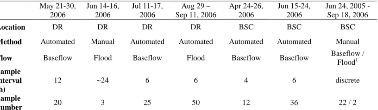
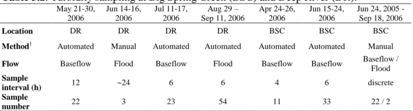
We compared short-term (3-10 days) and long-term (Apr-Sep) changes in OWQ during baseflow and flood conditions at DR and BSC to assess temporal trends (Table 1). Automated samples were collected in acid-washed bottles using Teledyne-ISCO 6712 autosamplers. Manual samples were collected following the same protocol as section 4.1.1. All samples were kept dark and refrigerated at ~4oC until analysis. Water
chemistry and OWQ analyses were performed within 72 h of sample collection, with only two exceptions (2 flood samples for BSC).
4.2. Hydrology
We obtained 15-minute discharge records from the USGS gages #05405000 and #05407000 for BR and WR, respectively (Figure 1). Discharge records for BSC and DR were obtained from stage-Q rating curves we developed using 15-min water-level
readings from stage recorders (Intech WT-HR 2000 for BSC and HOBO 9 m for DR) and in-situ Q measurements taken with a Marsh-McBirney current meter at the sampling sites.
4.3. Water Chemistry
Turner Designs TD-700 fluorometer according to APHA Standard Methods procedure 10200H (APHA 1998) using Whatman GF/F glass fiber filters. For WR, we measured chl-a with a Beckman DU Series 600 UV/VIS spectrophotometer according to Hauer and Lamberti (1996).
4.4. Optical Measurements 4.4.1. Turbidity
We measured turbidity (Tn) with a Hach 2100P turbidimeter in nephelometric
turbidity units (NTU), which is a relative measure of b (Kirk 1994). We used the average value of three Tn measurements for each sample, thoroughly mixing the sample prior to
each measurement.
4.4.2. Inherent Optical Properties (a, b, and c)
We used a Beckman DU Series 600 UV/VIS spectrophotometer to determine the inherent optical properties of the water samples. The spectrophotometer measured the amount of incident radiant flux (Ф0) that was received by a light detector (Ф) after being
incident light that was left after absorption and scattering by the water sample. By transforming Equation 2 and using the TCH, c was calculated as follows:
c = -ln(Ф/Ф0)TCH/r (2.5)
We derived the absorption coefficient (a) by using a Beckman standard cell holder (SCH), which placed the water sample 10 mm from the light detector and increased the collection angle to 14o. This large collection angle and close proximity of the water sample to the detector ensured that almost all scattered light was detected, thus quantifying only the absorption by the water sample (Davies-Colley et al. 2003).
Residual scattering not captured by the light detector was corrected for by subtracting out the apparent absorption coefficient at 740 nm (Χ740) because essentially all measured
absorption at 740 nm is due to scattering (Davies-Colley et al. 2003). Using the SCH, a was calculated as follows:
Χ = -ln(Ф/Ф0)SCH/r (2.6)
a = Χ – Χ740 (2.7)
where Χ is the apparent absorption coefficient for the measured wavelength. Equation 7 assumes that the angular range of scattering for the desired wavelength is the same as that at 740 nm. Using equation 1, we calculated the scattering coefficient (b) by subtracting a from c, as recommended by Davies-Colley, et al. (2003).
4.4.3. Spectrophotometer Scans
derive the variables in equations 5 – 7 and partition c (described below), we performed four configurations of scans on each water sample (Figure 2): TCH-UF (turbidity cell holder, unfiltered sample), TCH-F (turbidity cell holder, filtered sample), SCH-UF (standard cell holder, unfiltered sample), SCH-F (standard cell holder, filtered sample). We performed 3 scans for each configuration and used mean values for subsequent analyses. From the spectrophotometer scans, we used readings at 440 nm (index of CDOM), 740 nm (residual scattering), and the average of 400 -700 nm (PAR). Unless denoted by a subscript identifier (e.g., a440), all reported attenuation coefficients are
average values for PAR.
We also used the spectrophotometer scans to compare OWQ between the four study sites and to previous studies. The spectrophotometer scans (Figure 2) illustrate the change in absorbance (D) with wavelength (λ), where:
D = log10 (Ф0/Ф) (2.8)
The magnitude of the absorbance at 740 nm illustrates the degree of scattering in the water column (Figure 2), which indicates the concentration of particulates since scattering by dissolved constituents is negligible. The magnitude of the absorbance at 340 nm illustrates the degree of absorption in the water column (Figure 2), which indicates the CDOM concentration since absorption of light by CDOM increases
SCH-UF absorbance curve at 675 nm (Gallegos and Neale 2002), which is an absorption peak of chl-a (Figure 2).
4.5. Partitioning the Light Attenuation Coefficient
We partitioned the light attenuation coefficient into its constituent fractions (Equation 4) by using combinations of TCH vs. SCH and UF vs. F (Table 2). Using the TCH on an unfiltered sample quantifies the collective light attenuation coefficient by the dissolved (cd) and particulate (cp) constituents. Because the spectrophotometer was
blanked with Milli-Q water prior to measurements, we added the attenuation coefficient of pure water (cw) to the TCH-UF reading to obtain the total light attenuation coefficient
(c). Values for cw, aw, and bw were obtained from the data of Buiteveld, et al. (1994).
Using the SCH on an unfiltered sample quantifies the collective light absorption coefficient by the dissolved (ad) and particulate (ap) constituents. We added the
absorption coefficient of pure water (aw) to the SCH-UF reading to obtain the total light
absorption coefficient (a). Using the TCH on a filtered sample quantifies cd. Using the
SCH on a filtered sample quantifies ad. We derived particulate attenuation coefficients
by subtracting the dissolved and water attenuation coefficients from the total attenuation coefficients (Equation 4). For example, cp = c – cd – cw (TCH-UF – TCH-F, Table 2).
We derived scattering coefficients by subtracting the absorption coefficients from the attenuation coefficients (Equation 1).
We partitioned cp into cSS and cPOM by using the ap and bp of water samples where
usually negligible, ap for any water sample can be attributed entirely to POM (ap = aPOM).
Given that bPOM = Κap, where Κ is bPOM/aPOM , the light attenuation coefficient of POM
(cPOM) can be approximated with:
cPOM = aPOM + bPOM = ap + Κap (2.9)
This equation assumes that Κ is a constant for all POM in the water column. It also assumes that cPHYTO is negligible or either incorporated into cPOM.
4.6. Optical Water Quality Budget
We quantified the effect of tributaries on spatial trends in OWQ by creating an OWQ budget for the Baraboo River using the additive principle suggested by Davies-Colley, et al. (2003):
cdsQds = cusQus + ctribQtrib (2.10)
where c is the light attenuation coefficient in m-1, Q is discharge in m3/s, and the
subscripts ds, us, and trib denote downstream, upstream, and tributary, respectively. This method assumes that OWQ is volume conservative, where constituents do not experience physical or chemical changes (e.g., sedimentation of SS) between the upstream and downstream sites. To obtain c, we used Equation 5 on water samples collected from seven confluences. At each confluence, we sampled immediately upstream of the confluence (cus), at the tributary outlet before it entered the mainstem channel (ctrib), and
below the confluence before any other tributaries entered the mainstem channel (cds). Q
hydrography data (1:24,000 scale) to characterize stream-link magnitudes (i.e., stream order via the Strahler method; (Gordon et al. 2004)). “Major” tributaries (sensu Benda et al. 2004) were identified on the basis of a stream order greater than or equal to n – 1, where n is the stream order of the mainstem channel before the confluence.
4.7. Synoptic Optical Water Quality Datasets
We assessed longitudinal trends in OWQ by comparing our two longitudinal OWQ profiles from BR and WR with published synoptic OWQ datasets that met two conditions: (i) OWQ was measured in at least five locations from near the headwaters to the river’s mouth; and (ii) the mainstem channel was greater than 100 km. Three datasets fulfilled these criteria, all from New Zealand: Motueka River (110 km; Davies-Colley 1990), Pomahaka River (147 km; Harding et al. 1999), and Waikato River (330 km; Davies-Colley 1987). The Waikato R. study measured secchi disk depth (zSD), which we
converted to c using the method of Gordon and Wouters (1978; c = 6/zSD). The
Pomahaka R. and Motueka R. studies measured black disk visibility (yBD), which we
converted to c using the method of Davies-Colley (1988; c = 4.6/yBD for rivers). We used
these five synoptic OWQ surveys to test the prediction of the RCC (Vannote et al. 1980) that optical water quality decreases (i.e., c increases) along the river continuum from headwaters to mouth.
5. RESULTS
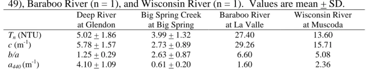
Big Spring Creek (BSC) had the highest OWQ (i.e., most optically clear) because of its low SS, POM, DOC, and PHYTO (Table 3). These characteristics caused the water of BSC to be essentially colorless because of the lack of scattering or absorption of light. BSC had the lowest average baseflow c at 2.73 + 0.89 m-1 (mean + std. dev.) and the lowest average baseflow Tn at 3.99 + 1.32 NTU of the four study sites (Table 4). Deep
River (DR) had a yellowish hue due to preferential blue-light absorption by its high DOC concentration. The average baseflow c and Tn for DR was 5.78 + 1.57 m-1 and 5.02 +
1.86 NTU, respectively. Wisconsin River (WR) at Muscoda also had a yellowish hue due its high DOC concentration (Table 3). The c and Tn for WR at Muscoda were 15.71
m-1 and 13.6 NTU, respectively. Baraboo River (BR) at La Valle had the lowest OWQ predominantly because of high SS and POM (Table 3) which imparted a dark-brownish hue on the water. This site had the highest c and Tn of the four study sites at 29.26 m-1
and 27.40 NTU, respectively.
Spectrophotometer scans of baseflow samples illustrated the relative differences in OWQ among the four study sites (Figure 3). BR had the highest TCH-UF absorbance curve at 740 nm and thus had the highest total scattering coefficient (b) at 25.41 m-1, followed by WR at 13.13, DR at 4.39, and BSC at 2.53. We found a strong correlation between TSS (SS + POM; Table 3) and b (r2 = 0.98, p = 0.027), which supports the relationship of increased scattering with increased concentration of particulates. DR had the highest SCH-F absorbance curve at 340 nm and thus had the highest CDOM
absorption coefficient (a440) at 4.44 m-1, followed by WR at 2.36, BR at 1.60, and BSC at
0.41. DOC explained 82% of the variance in a440, although the regression was not
At all four sites, scattering was the dominant process of light attenuation (b/a > 1), with BR having the highest b/a at 6.60, followed by WR at 5.08, BSC at 4.10, and DR at 1.64. The magnitude of light attenuation by PHYTO was negligible at DR and BSC because of the lack of a shoulder at 675 nm in the SCH-UF absorbance curves (Figure 3). Their low chl-a concentrations (Table 3) support this result. BR and WR had small shoulders at 675 nm due to higher chl-a (Table 3). However, the height of the shoulders relative to the magnitude of the absorbance curves for these sites was small, which results in minimal contribution of PHYTO to light attenuation.
Turbidity was a highly significant (p < 0.001) predictor of c at all four sites (Figure 4). The plots for DR and BSC (Figure 4A, B) represent changes in c and Tn in
response to changes in Q at-a-station; whereas, the plots for BR and WR (Figure 4C, D) represent longitudinal changes in c and Tn throughout the basin.
5.2. Temporal Trends: Deep River and Big Spring Creek 5.2.1. Turbidity and Discharge
Turbidity generally increased with increasing Q for DR and BSC (Figure 5). Q explained 77% of the variance in Tn at DR (Figure 5B; p < 0.001). We attribute the
variance to hysteresis, inter-storm, and seasonal effects. For example, Tn values for the
and Q at DR (r2 = 0.71; c = 1.43Q1.04) was similar to the relationship between Tn and Q
(Figure 5B).
Discharge explained only 27% of the variance in Tn at BSC (Figure 5D; p <
0.001). We attribute most of the variance to seasonal effects. The reduced vegetative ground coverage of BSC basin during the winter allowed greater surface sediment runoff, especially during the numerous snowmelt runoff events that occurred in central
Wisconsin during the 2005-2006 winter. This scenario is the likely cause of the two high Tn measurements in March 2006 (Figure 5C). The other considerable seasonal effect on
Tn in BSC was the die-off of in-channel vegetation during the late-summer. BSC had a
dense benthic coverage of aquatic macrophytes, which began to senesce in late-July (Zahn 2007). This senescence not only added plant fragments to the water column, but also fine sediment that was previously trapped by the vegetation. This scenario is the likely cause of the increasing Tn values starting in August of both years (Figure 5C).
Another contributing factor to increased Tn at BSC was bioturbation, with the greatest
turbidity pulses being caused by cows and geese. The extremely high Tn in Feb. 2006 (64
NTU, Figure 5C) was most likely caused by one of these two animals. The relationship between c and Q at BSC (r2 = 0.43; c = 1370.9Q4.85) was similar to the relationship between Tn and Q (Figure 5D).
5.2.2. Baseflow OWQ of Big Spring Creek
The OWQ of Big Spring Creek varied relatively little during the 10-day baseflow period from June 15 – 24, 2006 (Figure 6A). Particulates (cp: 81%) accounted for most
The particulates consisted of 47% POM (2.2 mg/L) and 53% mineral sediment (2.7 mg/L). The concentration of chl-a was relatively low and constant over the 10 days (6.3 + 1.0 µg/L). The baseflow period of BSC was characterized by small and brief pulses of SS, POM, and CDOM. Overall, CDOM (a440) remained fairly constant at 0.67 m-1 and
TSS decreased from 5.4 to 3.4 mg/L. The decrease in TSS was therefore the cause for the decrease in c over the 10-day period, from 3.3 to 2.0 m-1 (Figure 6A).
5.2.3. Baseflow OWQ of Deep River
The OWQ of Deep River increased (i.e., c decreased) slightly during the 10-day baseflow period from May 21 – 30, 2006 (Figure 6B). During this baseflow period, cp
accounted for most (64%) of the light attenuation, followed by cd (33%) and cw (3%;
Figure 6B). The particulates consisted of 34% POM (2.1 mg/L) and 66% mineral sediment (4.1 mg/L). The concentration of chl-a was minimal and relatively constant over the 10 days (1.2 + 0.1 µg/L). The baseflow period of DR was characterized by decreases in SS (5.6 to 2.9 mg/L) and CDOM (4.4 to 2.2 m-1), resulting in a decrease of c from 6.7 to 3.6 m-1 (Figure 6B). During this time, POM % increased at an average rate of 3.0% per day (20 to 50%). TSS, however, remained fairly constant at 6.3 mg/L,
suggesting that sediment was settling out while additional sources of POM were being added to the water column. During the other baseflow sampling period (July 11 – 17, 2006; data not illustrated), POM % increased at an average rate of 4.5% per day (20 to 47%) while TSS remained fairly constant at 7.6 mg/L.
In contrast to the limited change in OWQ during baseflow, the magnitude and composition of c varied greatly through a flood at DR on Aug 30, 2006 (Figure 6C; Qpeak
= 60 m3/s, recurrence interval (RI) of ~2 months). This flood occurred following a prolonged (~1 month) low-flow period (Figure 5A) and thus pre-flood water column concentrations of TSS (3.0 mg/L) and CDOM (2.7 m-1) were relatively low. Before the flood, c was 3.5 m-1, with cp accounting for most light attenuation (60%), followed by cd
(35%) and cw (5%). Pre-flood POM averaged 87% of TSS. The value of c increased
rapidly during the rising limb of the flood due mostly to a pulse of TSS, and c reached a maximum of 137.3 m-1 at 12 hours after Qpeak. This lag was caused by an additional TSS
pulse, which was most likely from a tributary with a slower travel time. As particulates settled out of the water column following Qpeak, c decreased exponentially until it reached
its average baseflow value of 5.8 m-1 at 8 days following Qpeak. CDOM also increased in
response to the flood and maintained elevated concentrations during the entire sampling period, which is characteristic of subsurface flow following a dry period (Walling and Webb 1992). Consequently, the relative proportion of light attenuation by CDOM increased following the flood, reaching a maximum of 53% (Figure 6C).
5.2.5. Components of Optical Water Quality
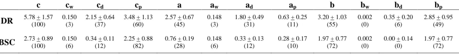
Partitioning the total light attenuation coefficient (c) by means of Equation 4 and Table 2 revealed that scattering by particulates (bp) was the dominant process of
mid-summer baseflow light attenuation at DR and BSC (Table 5). Absorption by CDOM (ad)
and particulates (ap) were the two other main contributors to baseflow light attenuation at
m-1, of which 82% was from TSS (cp), 12% from CDOM (cd), and 6% from water (cw).
For all combined baseflow sampling at DR, c averaged 5.78 + 1.57 m-1, of which 60% was from TSS (cp), 37% from CDOM (cd), and 3% from water (cw).
Using water samples where TSS was 100% POM, we found that bPOM/aPOM (or K;
see Section 4.5.) for DR was ~3 (3.06 + 0.65, n = 5). There were no water samples from BSC where TSS was 100% POM, and therefore we used K from DR for BSC. Assuming that K equals 3, the light attenuation coefficient of POM (cPOM) is approximately 4ap
(Equation 9). Using Equation 9 and Table 5, we calculated the amount of baseflow light attenuation by water, CDOM, SS, and POM at each site (Figure 7). Light attenuation by PHYTO was included in POM, but given its low concentrations at both sites (Table 3), its contribution to light attenuation was probably minimal. Vahatalo, et al. (2005) found that aPHYTO for the Neuse River basin, which is adjacent to the Deep River basin and had
slightly higher chl-a concentrations than DR, contributed 2.3 + 2.9% to a. During baseflow at DR, POM (43%) was the greatest contributor to light attenuation, followed by CDOM (37%), SS (17%), and water (3%; Figure 7). During baseflow at BSC, POM and SS both contributed 41% to total light attenuation, followed by CDOM (12%) and water (6%; Figure 7).
5.3. Spatial Trends: Baraboo River and Wisconsin River 5.3.1. Wisconsin River Continuum
associated with major tributary inputs and impoundments along this section of river (Figure 8B). Downstream of the last mainstem dam (RK 538), SS, POM, and PHYTO steadily increased, while CDOM remained fairly constant (Figure 8A). SS, POM, and PHYTO all reached their maximum values at the last sampling site (RK 674). The scattering to absorption ratio (b/a) along WR was highly irregular, ranging from 1.8 (RK 205) to 5.3 (RK 674), indicating large changes in SS and POM relative to CDOM
(Appendix 1).
The light attenuation coefficient (c) along WR followed a similar trend as SS and POM by fluctuating between 0.2 and 13.8 m-1 for the first 548 km and then steadily increasing after the last mainstem dam, reaching a maximum of 22.8 m-1 (Figure 8B, Appendix 1). There were two local peaks in c along WR, both of which occurred immediately downstream of confluences with turbid major tributaries. Between RK 250 and 292 (Big Rib River confluence at RK 256), c increased from 8.9 to 13.8 m-1.
Between RK 488 and 524 (Baraboo River confluence at RK 506), c also increased from 8.9 to 13.8 m-1 (Figure 8B). The c of BR before it entered WR was 25.2 m-1 (Figure 9B).
5.3.2. Baraboo River Continuum
therefore we relied on the shoulder height at 675 nm in the SCH-UF absorbance curve (index for PHYTO, Figure 2) to make inferences on its longitudinal distribution.
PHYTO was minimal in the headwaters (i.e., no shoulder), increased gradually to RK 40, and then decreased gradually toward the mouth of BR. This decrease in PHYTO at RK 40 coincided with a sharp increase in c (Figure 9B). The scattering to absorption ratio (b/a) increased along BR from 0.8 (RK 3) to 7.8 (RK 142), before decreasing to 5.9 at the mouth (RK 181) (Appendix 2). The increase in b/a was associated with increased
concentrations of SS and POM while CDOM remained relatively constant (Figure 9A). The decrease in b/a over the last 39 km of BR was associated with decreased
concentrations of SS and POM (Figure 9A) and lower channel gradient (Figure 9B), which indicates that the particulates were likely settling out of the water column over this reach.
The trend of c along the BR continuum was similar to that of SS and POM: (i) increasing gradually over the first 38 km; (ii) increasing rapidly over the next 34 km; (iii) increasing gradually over the next 70 km; and (iv) decreasing rapidly over the last 39 km (Figure 9B, Appendix 2). These trends in c matched the pattern of major confluences along BR, where c increased rapidly after three major confluences and began to decrease 40 km downstream of the last major confluence (Figure 9B). Also of note is that the local trough in c at RK 115 occurred immediately downstream of the confluence with the much clearer Narrows Creek (c = 16.63 m-1; Figure 10).
We used the synoptic OWQ and Q data through the BR watershed to develop an OWQ budget in which we quantified the relative influence of tributary OWQ (ctrib) on
mainstem OWQ (cus; Equation 10, Figure 10). All but two of the tributaries sampled
were major tributaries (Kratche Creek and Narrows Creek) and two of the major tributaries from Figure 9B were not sampled (Cleaver Creek at RK 25 and Seymour Creek at RK 34). Generally, ctrib and Qtrib increased in the downstream direction, which
is characteristic of greater drainage areas contributing greater amounts of SS and POM. The value of cus increased in the downstream direction for the first 73 km, but then
leveled off or decreased. The rate of increase in cus (0.38 m-1/km) over the first 73 km
was more than two times the rate of increase in ctrib (0.17 m-1/km), which resulted in an
OWQ inversion in which ctrib was greater than cus in the upper basin, but lower than the
cus in lower basin. Accordingly, the largest increase in c (+3.22 m-1) occurred in the
upper basin at the W. Branch Baraboo R. confluence, while the largest decrease in c (-4.82 m-1) occurred in the lower basin at the Narrows Cr. confluence (Figure 10).
The predicted product of cdsQds* (via Equation 10) and the actual product of
cdsQds (via Figure 10) agreed fairly well (Table 6). All predicted products were within
20% of the actual product, except the two uppermost confluences (Table 6). These two exceptions may have been caused by the greater variability in mixing/sedimentation processes in headwater streams, and/or the greater uncertainty of Q for small watersheds. The other five confluences suggest that OWQ in BR is generally volume conservative.
6. DISCUSSION
6.1.1. The Five Components
Optical water quality in rivers is dictated by the trends of five components: pure water, suspended sediment, particulate organic matter, chromophoric dissolved organic matter, and phytoplankton. The optical properties of pure water remain constant, and therefore its contribution to light attenuation decreases with increases in any of the other four components. Using a wide variety of rivers, we found that riverine OWQ is
primarily dictated by the particulates in the water column rather than by dissolved
constituents (Table 5, Appendix 1, 2). Our results are similar to Davies-Colley and Close (1990), who analyzed 96 New Zealand rivers during baseflow and found that 87% of the total light attenuation was attributed to particulates.
Our study also showed that during and immediately following floods, the
dominance of cp increases (Figure 6C) as SS and POM increase. The relative dominance
of SS vs. POM is likely to vary between (Figure 7) and within rivers (Figure 8A) due to source limitations. For example, the OWQ of rivers in the Midwest USA, such as BR, that drain areas with organic-rich soils and abundant vegetation is likely to be dominated by POM; whereas, the OWQ of rivers in the Southwest USA, such as the Colorado River, that drain areas of organic-poor soils and sparse vegetation is likely to be dominated by SS.
trends in CDOM are mostly influenced by the hydrologic regime of the river (Figure 6). Because most of the CDOM present in rivers is derived from terrestrial groundwater inputs (Webster et al. 1995, Wetzel 2001), the contribution of CDOM to light attenuation is usually greater following storms (via watershed flushing) and increases as particulates settle out of the water column (Figure 6C).
We did not quantify cPHYTO, but other riverine OWQ studies (Davies-Colley and
Close 1990, Duarte et al. 2000, Vahatalo et al. 2005) found that the contribution of PHYTO to light attenuation was either minimal or negligible over a wide range of rivers due to unfavorable conditions to phytoplankton growth. While particulates dominate OWQ for most rivers, there are exceptions, most notably in tidal and blackwater rivers (e.g., Gallegos 2005). In these rivers, PHYTO and CDOM have a much greater influence on OWQ. Future OWQ research opportunities can be directed towards determining if trends observed here hold for diverse types of rivers worldwide.
6.1.2. Optical Water Quality Measurements and Proxies
Riverine optical water quality has been measured using a variety of instruments, including a beam transmissometer Colley and Smith 1992), secchi disk (Davies-Colley 1987), black disk (Davies-(Davies-Colley 1990), and spectrophotometer (Vahatalo et al. 2005). While each method has its advantages and disadvantages (see Davies-Colley et al. 2003), we used a spectrophotometer because of its versatility. By using the
analyzed absorption (e.g., Vahatalo et al. 2005). However, this study (Table 5, Appendices 1 and 2) and others (Davies-Colley 1987) have shown the dominance of scattering on OWQ in rivers. Future spectrophotometric studies of riverine OWQ should use a method similar to ours (Figure 2, Table 2) in order to derive the total light
attenuation coefficient (c).
Despite the utility of the four-configuration spectrophotometer scan, the time, detail, and cost involved in such analyses may not make it a practical tool for water resource managers to assess riverine OWQ. We therefore recommend the use of turbidity (Tn) as a proxy for c. Comparisons of Tn and c showed that Tn is a strong predictor of c
(Figure 4), and data from studies of New Zealand rivers (Colley 1987, Davies-Colley and Smith 1992, Smith et al. 1997) produced similar relationships. While Tn
cannot be used to predict the exact value of c in unmeasured rivers, the strong correlation between c and Tn demonstrate that turbidity can be used to assess spatial and temporal
trends in OWQ for most rivers. The use of Tn as a proxy for c is advantageous because:
(i) there is a longer and more extensive record of Tn in rivers than c; (ii) Tn is easier and
less expensive to measure than c; and (iii) Tn is increasingly becoming a popular metric in
fluvial ecology studies. The use of Tn as a proxy for c is probably only valid for
non-tidal, non-blackwater rivers where scattering is the dominant process of light attenuation. In tidal and blackwater rivers, where absorption is likely to be the dominant process of light attenuation, other proxies such as CDOM or chl-a will need to be used.