Evaluating Latent Variable Interactions with Structural Equation Mixture Models
Ruth E. Mathiowetz
A thesis submitted to the faculty of the University of North Carolina at Chapel Hill in partial fulfillment of the requirements for the degree of Master of Arts in the Department of
Psychology.
Chapel Hill 2010
Approved by:
Daniel J. Bauer, Ph.D.
Robert C. MacCallum, Ph.D.
ii ABSTRACT
RUTH E. MATHIOWETZ: Evaluating Latent Variable Interactions with Structural Equation Mixture Models
(Under the direction of Dan Bauer)
Interactions are commonly hypothesized in psychological research. Methods exist for
estimating interactions with observed variables, but problems with small effect sizes,
measurement error, predictor distributions, and the unknown nature of the relationships
among the variables of interest make it difficult to detect interactions. Latent variable
approaches were proposed to remedy some problems with observed variables, however these
methods require a priori specification of the functional form of the interaction. The present
work evaluates an approach using structural equation mixture models (SEMMs) to estimate
interactions among latent variables without specifying a functional form in advance. Results
indicate that the approach can approximate a variety of latent variable relationships. Larger
sample sizes and areas with more observations were associated with better SEMM
performance. Typically, SEMMs with additional classes had less bias. It is recommended
that researchers examine predicted value plots for several SEMMs to evaluate the
iii
ACKNOWLEDGEMENTS
I would like to thank the members of the L.L. Thurstone Psychometric Laboratory for
creating an environment that challenges me to come up with new ideas and provides critical
feedback to help me refine them. I especially want to thank the members of Bauer Lab for
their guidance, encouragement and silliness along the way.
iv DEDICATION
To my ever supportive family and friends, including the one who told me, “This is an
v
TABLE OF CONTENTS
LIST OF TABLES……….……….…….. vii
LIST OF FIGURES……….………. viii
Chapter I. EVALUATING INTERACTIONS IN PSYCHOLOGY………..1
Linear Structural Equation Models………..…………...5
Parametric Approaches………..….…...7
Structural Equation Mixture Model Approach ………..…...11
Previous Studies Using Structural Equation Mixture Models………...….…14
Current study……….………....16
II. METHOD……….….…...19
Population Models………...19
Data Generation……….…...21
Model Fitting………..…...21
Evaluating Model Performance………...…..…...22
III. RESULTS……….…..…..…...26
Convergence and BIC Class Selection………...………26
Main Effects Model………..27
Nonlinear Model………...28
vi
Nonlinear Interaction Model………...36
Performance Across Data Generating Models………39
IV. DISCUSSION……….…...41
APPENDIX A: CONVERGENCE RATES AND BEST BIC
CLASS SELECTION ...………....71
APPENDIX B: ADDITIONAL PLOTS………...75
vii
LIST OF TABLES
Table
1. Best BIC class SEMM results the main effects condition ………..….…...48
2. One-class SEMM results for the main effects, skewed
data condition………...……..…49
3. Best BIC class SEMM results the nonlinear condition ………...50
4. Two-class SEMM results for the nonlinear condition……….………....51
5. Best BIC class SEMM results the bilinear interaction
condition ……….….…..52
6. Two-class SEMM results for the bilinear interaction
condition…………...53
7. Best BIC class SEMM results the nonlinear interaction
condition…………...54
8. Two-class SEMM results for the nonlinear interaction
viii
LIST OF FIGURES
Figure
1. Plot of 3-class SEMM for two dimensional SEMM example………...56
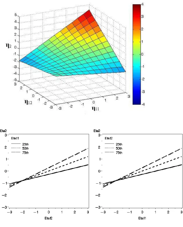
2. Plots of 2-class SEMM for three-dimensional SEMM example………...57
3. Plots of the expected values for the main effects model………..……….58
4. Plots of the expected values for the nonlinear model………...59
5. Plots of the expected values for the bilinear interaction model………....60
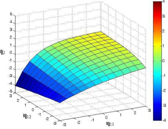
6. Plots of the expected values for the nonlinear interaction model……….61
7. Estimated average surface plots for the main effects condition…………...62
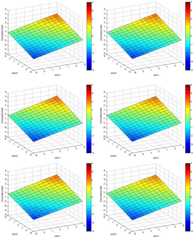
8. Estimated average surface plots for the nonlinear condition………63
9. Simple slope plots for the nonlinear condition……….64
10. Example estimated average surface and bias surface plots for the bilinear interaction condition………....65
11. Example estimated surface and discrepancy surface plots for one replication from the bilinear interaction condition………..66
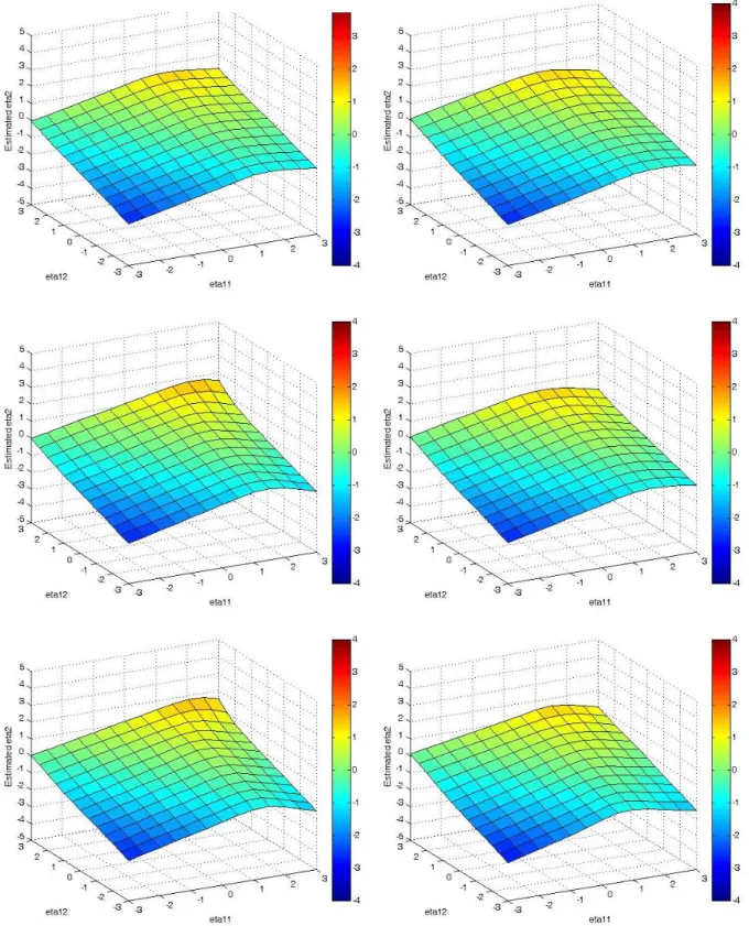
12. Estimated average surface plots and bias surface plots for the bilinear interaction condition………..67
13. Simple slope plots for the bilinear interaction condition……….68
14. Estimated average surface plots and bias surface plots for the nonlinear interaction condition ………...69
Chapter 1
EVALUATING INTERACTIONS IN PSYCHOLOGY
Researchers often hypothesize that independent variables have both main effects and
interaction or moderation relationships with a dependent variable. For example, an
information processing theory proposes that motivation interacts with ability to influence
performance (e.g. Humphreys & Revelle, 1984). Many researchers have also posited
gene-environment interaction theories (e.g. Tryon,1940; Scarr, & McCartney, 1983). A third
example is Double-Jeopardy Theory which hypothesizes that individuals with multiple
subordinate-group identities (e.g. low SES and female) suffer more discrimination than
individuals who are members of only one subordinate-group identity (e.g. Beal,1979;
Purdie-Vaughns, & Eibach, 2008) These examples show how interactions are a component of many
psychological theories.
Methods for testing and probing interactions are well articulated in textbooks (e. g.
Maxwell & Delaney, 2004; Aiken & West, 1991) and are often implemented in
psychological studies (e.g. Blackwell, Trzesniewski, & Dweck, 2007; Peterson, Haynes, &
Olson, 2008; Bergstrom, Neighbors, & Malheim, 2009). However, several authors have
noted that it can be challenging to detect statistically significant interactions with observed
variables (Busemeyer & Jones, 1983; Baron & Kenny, 1986; Chaplin, 1991; McClelland &
Judd, 1993). One problem with detecting interactions with observed variables is the effect
size of the interactions that are typically found in psychological studies. In his study of
2
are likely to be very small (e.g. a partial correlation between the criterion and the interaction
term of around .1). He argued that with such a small effect size researchers need to have a
large sample size and low measurement error to provide sufficient power to detect
interactions. Prior to Chaplin‟s (1991) work, Busemeyer and Jones (1983) demonstrated how
having measurement error decreases the likelihood of accurately detecting interactions with
observed variables. Specifically, their work showed that measurement error attenuates the
relationships among observed variables, leading to the underestimation of interaction and
higher order trends.
Besides small effect size and measurement error, McClelland and Judd (1993)
provided evidence that low power to detect interactions may also be related to the
distributions of the predictors. Using simulated data, they showed that having observations in
the extremes of the distributions of the predictors increases the power to detect interactions.
One reason that researchers may fail to detect interactions with non-experimental data may
be that too few observations occur at the extremes.
Another significant issue when trying to detect interactions is that researchers often
do not know the form of the interaction (e.g. crossover, fan-shaped). McClelland and Judd
(1993) found the nature of the interaction contributes to the possibility of detection. They
showed that cross-over shaped interactions are easier to detect than fan shaped interactions.
In addition to the unknown interaction form, researchers may not know the functional form
(e.g. linear, quadratic, exponential) of the relationships among the variables of interest.
Busemeyer and Jones (1983) showed how the unknown functional form of the model can
decrease the likelihood of accurately detecting interactions with observed variables. They
3
nonlinear trend can result in spurious interaction effects. The results of these studies show
that the lack of knowledge about the functional form of the relationships among a set of
observed variables makes it difficult for researchers to be confident that they have correctly
specified any given model and that any interaction effects found are not spurious.
Latent variable models or structural equation models (SEM) have been proposed as a
potential approach to address some of these problems. Kenny and Judd (1984) proposed
using SEM to estimate interactions with latent variables in order to account for the
measurement error found in observed variables. Baron and Kenny (1986) offered additional
support for using an SEM approach by arguing that SEM can reduce the problem of
unreliable measurement by using multiple indicators to measure a construct. They also noted
that SEM can test all of the relationship paths of interest simultaneously and has enough
flexibility to be used with both experimental and non-experimental data. The main drawback
of SEM is that it was developed to estimate linear relationships among observed and latent
variables. The need to estimate nonlinear relationships or interactions among latent variables
therefore required the development of modeling methods that could circumvent the
assumption of linearity.
The issue of linearity is less problematic for categorical moderators, and several SEM
techniques have been developed for evaluating latent variable interactions with categorical
variables, such as tests for model invariance over multiple groups (Rigdon, Schumaker &
Wothke, 1998; Bollen, 1989). However, methods for estimating interaction models with
continuous latent predictors have been more challenging to develop because in addition to
the nonlinearity, the product variable representing the continuous variable interaction is
4
formed when taking the product of two normally distributed exogenous latent variables. This
non-normal distribution violates the normality assumption of some SEM estimators.
Many approaches for estimating continuous latent variable interactions have been
proposed, some that try to estimate the latent product interaction with indicators and others
that attempt to estimate it directly. Several product-indicator approaches have been
developed with various nonlinear constraints on the covariance matrix and methods to
account for the non-normal distribution of the interaction variable (Ping, 1995; Jöreskog &
Yang, 1996; Algina & Moulder, 2001; Wall & Amemiya, 2001). Other approaches tried to
account for the non-normality of the latent product by using Bayesian methods (Arminger &
Muthén, 1998; Zhu & Lee, 1999) or variations of maximum likelihood (Klein &
Moosbrugger, 2000; Klein & Muthén, 2007). In addition to these methods that assume
specific distributions, several distribution-free approaches have been proposed, including a
two-stage least squares estimator (Bollen & Paxton, 1998) and a method of moments
estimator (Wall & Amemiya, 2003).
All of these approaches require good theory to justify the functional form of the
interaction, many can be tedious to specify and some require normally distributed latent
predictors (precisely the case that McClelland and Judd (1993) noted leads to low power). It
is important to note that although these procedures offer viable solutions to the problem of
measurement error, none address the issue that the functional form of the relationship
between the outcome and predictors is often unknown. Each of the above procedures
assumes a bilinear or product interaction, which Busemeyer and Jones (1983) found to be
5
Recently, Bauer (2005) proposed an alternative, semiparametric approach that does
not assume a bilinear interaction. This approach uses a mixture of linear structural equation
models. Relationships are thus assumed to be locally linear, within mixing components.
Nonlinear relationships are recovered by averaging over the mixing components. The
structural equation mixture model (SEMM) approach offers a way to estimate interactions
that (a) accounts for measurement error with latent predictors, (b) allows for latent predictors
with non-normal distributions (assuming these distributions to be a finite mixture of normals)
and (c) estimates nonlinear relationships without assuming a specific functional form.
To better contrast the SEMM approach to previous methods I will describe the
traditional linear SEM and parametric methods for estimating latent variable interactions in
greater detail, and then provide background information on the SEMM approach. Finally, I
will address the need to demonstrate the utility of this approach and propose a simulation
study to examine the conditions under which the approach can be successfully implemented.
Linear Structural Equation Models
The structural equation model is designed to estimate linear relationships among
observed and latent variables. It is composed of two parts. The first part is a measurement
model, which contains the equations relating the observed variables to their latent constructs.
The second part is a latent variable model, which contains the linear relationships among the
latent constructs. The measurement model for the observed variables can be written as
𝒚𝑖 = 𝝂 + 𝜦𝜼𝑖 + 𝜺𝑖 𝜺𝑖 ~ N(𝟎, 𝚯) (1)
Where 𝒚𝑖 is a vector of observed variables for individual i. The measurement intercepts are
6
the relationships between the latent variables found in 𝜼𝑖 to the observed variables. The
measurement error for individual i is represented by 𝜺𝑖.
The structural or latent variable model is given as
𝜼𝑖 = 𝜶 + 𝜷𝜼𝑖+ 𝜻𝑖 𝜻𝑖 ~ N(𝟎, 𝚿) (2)
Where 𝜼𝑖 is the vector of latent variables, 𝜶 is the vector of latent intercepts, 𝜷is the matrix
of regression coefficients that contains the relationships among the latent variables and 𝜻𝑖 are
the residuals.
Based on Equation 1 and 2 the mean vector 𝝁 𝜽 and covariance matrix 𝜮 𝜽 for the
model are parameterized as
𝝁 𝜽 = 𝝂 + 𝜦(𝑰 − 𝜷)−1𝜶 (3)
𝜮 𝜽 = 𝜦(𝑰 − 𝜷)−1𝝍(𝑰 − 𝜷)−1𝜦′+ 𝜣 (4)
The formulas for the SEM show the linear relationships among the observed and latent
variables. Specifically, Equation 2 does not include interaction relationships among the latent
variables (𝜼𝑖). In addition to not including interaction relationships in the structural model,
several other problems arise when trying to include latent variable interactions in SEMs. To
include a product interaction would violate the assumption of some SEM estimators that the
latent predictors are normally distributed, because the product distribution of two normal
distributions is not normal. Additionally, it is unclear how the interaction term would be
measured as there are no observed variables that directly measure the interaction. Products of
the indicators for the latent variables involved in the latent interaction could be included, but
that would violate the assumption of normally distributed indicators. Potential solutions to
7 Parametric Approaches
Kenny and Judd (1984) provided the first widely used method to estimate latent
variable interactions using product indicators. They formed indicators for a latent interaction
variable by taking products of the indicators from the two latent exogenous variables. For
example, with two latent predictors measured by two indicators each, the measurement
model would be extended to include the product indicators, which would be expressed as
𝑥11 𝑥12 𝑥21 𝑥22 𝑥11𝑥21 𝑥11𝑥22 𝑥12𝑥21 𝑥12𝑥22 𝑦
=
1 0 0 0 𝑔 0 0 0 0 1 0 0 0 0 0 0 0 1 0 0 0 0 0 0 𝑔 0 0 0 𝑔 0 0 0 1 0
𝜉1 𝜉2 𝜉1𝜉2
𝜂1 + 𝜀1 𝜀2 𝜀3 𝜀4
𝜀1𝜀3+ 𝜉1𝜀3+ 𝜉2𝜀1 𝜀1𝜀4+ 𝜉1𝜀4+ 𝜉2𝜀1 𝜀2𝜀3+ 𝑔𝜉1𝜀3 + 𝜉2𝜀2 𝜀2𝜀4+ 𝑔𝜉1𝜀4 + 𝜉2𝜀2
𝜀5
(5)
Where ξ1and ξ2 are the latent exogenous variables and ξ1ξ2 represents the latent exogenous interaction. The latent endogenous variable is η1 and the observed indicator variables are
𝑥11, 𝑥12, 𝑥21, 𝑥22 and 𝑦. The product indicators are represented by 𝑥11𝑥21, 𝑥11𝑥22, 𝑥21𝑥21
and 𝑥21𝑥22. This matrix form for the Kenny-Judd measurement model illustrates how the
approach constrains the relationships among the latent variables.
The structural model for the Kenny-Judd approach would be parameterized as
𝜂1 = 𝛽1 𝛽2 𝛽3 0 𝜉1 𝜉2 𝜉1𝜉2
𝜂1
+ 𝜁 (6)
The only difference between the traditional SEM structural model shown in Equation 2 and
the Kenny-Judd structural model in Equation 6 is the addition of a product latent variable for
8
In this specification of the interaction model, the latent variables (𝜉1, 𝜉2 and 𝜂1) as
well as the observed indicators are assumed to be normally distributed. Because several SEM
estimators assume normally distributed latent variables, the model requires complex
nonlinear constraints to be specified in the covariance matrix. These nonlinear constraints are
necessary to estimate the model parameters for the product variables (e.g. the variance of the
product indicators) and they lead to fewer new parameters to estimate when adding an
interaction to the model. The disadvantages of the nonlinear constraints are that they are not
easily implemented and they are based on the assumption that the indicators are normally
distributed (prior to taking the products), which may not be appropriate in some situations.
Besides the problems associated with the normality assumption for the latent
variables, the assumption that the indicators are normally distributed can also be problematic.
First, because the indicators are assumed to be normally distributed, the product indicators
are non-normally distributed. Thus, in order to estimate the interaction, an SEM estimation
procedure that does not assume multivariate normality must be used. Kenny and Judd (1984)
used a generalized least squares estimation procedure that did not provide standard errors for
the parameter estimates, which prevented the creation of confidence intervals or significance
testing. Given the limitations of their model, Kenny and Judd (1984) viewed their approach
as a “partial solution” to the problem of estimating interactions among latent variables.
Several subsequent papers as well as a book edited by Schumacker and Marcoulides
(1998) on estimating interaction and nonlinear effects in SEM offered improvements to the
Kenny-Judd method. Many papers were concerned with implementation issues, for instance
how to specify the method in LISREL (Hayduk, 1987; Jaccard & Wan, 1996), or implement
9
Yang, 1996). Other implementation papers focused on how many product indicators to use
(Jöreskog & Yang, 1996; Marsh, Wen & Hau, 2004) or how the product indicators are
constructed (Marsh, Wen & Hau, 2004; Saris, Batista-Foguet & Coenders, 2007). An
important contribution from Jöreskog and Yang (1996) showed how to implement the
procedure with mean structure and noted that results could be biased if the mean structure
was not included. Unfortunately, the addition of mean structure increased the number of
constraints required to implement the model.
In response to the complication of implementing the Kenny-Judd approach, Ping
(1995, 1996) proposed a two-step estimation approach to calculate the latent interaction
variable without some of the complex nonlinear constraints of the Kenny-Judd method.
Besides Ping‟s two-step approach, several other papers addressed the issue of how to specify
the model constraints. Algina and Moulder (2001) proposed what would later be referred to
as the „constrained‟ approach, including the mean structure of Jöreskog and Yang (1996), but
with the additional model constraint of using population mean-centered predictors to improve
convergence rates. Bollen and Paxton (1998) proposed the two-stage least squares (2SLS)
approach, which was a distribution-free method that used instrumental variables to eliminate
the assumption of normally distributed indicators and the associated covariance matrix
constraints. Unfortunately, this approach was found to be inefficient, compared to other
procedures (Scherelleh-Engel, Klein & Moosbrugger,1998; Moulder & Algina, 2002).
Similarly, Wall and Amemiya‟s (2001) GAPI approach also removed the assumption of the
normally distributed indicators, but kept some of the nonlinear constraints of the Kenny-Judd
approach. Likewise, the „unconstrained‟ approach of Marsh, Wen and Hau (2004) relaxed the
10
constraints of the Kenny-Judd approach. By eliminating some of the distributional
assumptions and constraints from the Kenny-Judd approach, both the GAPI and the
„unconstrained‟ approaches offer easier model specification and allow for non-normally
distributed indicators and latent predictor variables.
Because the product indicator approach is somewhat ad hoc, several alternatives to
these approaches were proposed to directly estimate the interaction without product
indicators. These approaches include a latent moderated structural (LMS) equations approach
(Klein & Moosbrugger, 2000), a quasi-maximum likelihood (QML) approach developed by
Klein and Muthén (2007) and the Bayesian methods found in Arminger and Muthén (1998),
Zhu and Lee (1999) and Lee et al. (2007). In addition, Wall and Amemiya (2003) proposed a
two-stage method of moments (2SMM) procedure that first obtains factor scores from the
measurement model and then fits the latent variable model based on the factor scores. By
avoiding the use of product indicators, these alternative procedures eliminate the complex
nonlinear constraints and the associated distributional assumptions required for many of the
product-indicator approaches.
It is important to recognize that both the product-indicator and alternative approaches
to estimating interactions offer several potential solutions to the problems of measurement
error and distributional assumptions. By using latent variables these methods remove the
threat of measurement error attenuating relationships among variables and thereby increase
the likelihood of detecting interactions. Besides accounting for measurement error, many of
these models have been developed to account for non-normally distributed latent variables
11
variables would likely lead to low power to detect interactions, so having methods that can
handle non-normal data should be important for detecting interactions.
Although these methods address two major issues with the estimation of interactions,
measurement error and distributional assumptions, none of these approaches addresses the
issue of functional form. These methods are parametric because one must assume a
functional form for the interaction, usually a bilinear or product interaction. This assumption
may not be justifiable. Busemeyer and Jones (1983) demonstrated the problems that can
arise if the functional form of the interaction is incorrectly specified. Given their findings, it
would be useful to have a method that does not assume a specific form for the interaction.
Structural Equation Mixture Model Approach
Unlike the parametric approaches, the semiparametric SEMM approach was proposed
to account for measurement error and to allow for non-normal latent variable distributions,
while not assuming a functional form of the interaction. The SEMM is an extension of the
traditional linear SEM. The SEMM allows a linear SEM (described in Equations 1 and 2) to
be fit across K latent classes where each class is characterized by a normal component
distribution with its own mean vector, 𝝁 𝜽𝑘 , and covariance matrix 𝜮(𝜽𝑘). By averaging
over the within-class linear SEMs (using the conditional probability of class membership)
one can approximate nonlinear relationships, such as an interaction. To better illustrate this
process I will first explain the parts of the general SEMM, then show how an SEMM can be
used to recover a nonlinear relationship among two latent variables (two-dimensional case). I
will also provide an example where two latent predictor variables interact to influence a third
latent outcome variable (three-dimensional case). Lastly, I will provide details regarding the
12
An examination of the probability density function (PDF) of SEMM reveals how the
model is a mixture of normal distributions. The SEMM PDF is given as
𝑓 𝒚 = 𝐾 𝑃 𝑘 𝜑𝑘[𝒚; 𝝁 𝜽𝑘 , 𝜮(𝜽𝑘)]
𝑘=1 (7)
where 𝑃 𝑘 represents the mixing probability for the class k and the sum of the class
probabilities is 1. Within each class, the observed variables represented by y follow a
multivariate normal distribution, indicated by 𝜑𝑘, with a mean vector of 𝝁 𝜽𝑘 and
covariance matrix 𝜮(𝜽𝑘), which are parameterized as 𝝁𝑘 𝜽𝑘 = 𝝂𝑘 + 𝜦𝑘(𝐈 − 𝜷𝑘)−1𝜶
𝑘 (8)
𝜮𝑘 𝜽𝑘 = 𝜦𝑘(𝑰 − 𝜷𝑘)−1𝝍
𝑘(𝑰 − 𝜷𝑘)−1𝜦𝑘′+ 𝜣𝑘 (9)
The subscript k indicates matrices that can potentially vary across class. In practice many of
these matrices may be constrained to be the same across classes, both to ease estimation and
improve interpretability.
The first step for applying the SEMM approach is to restructure the matrices to
separate the latent exogenous variables,𝜼1, from the latent endogenous variables, 𝜼2, such
that the new matrices are given as:
𝜼′= 𝜼1′ 𝜼
2
′ (10)
𝜶′= 𝜶1𝑘′ 𝜶
2𝑘
′ (11)
𝜷𝑘 = 𝜷𝟎 𝟎
21𝑘 𝟎 (12)
𝝍𝑘 = 𝝍𝟎11𝑘 𝝍𝟎
22𝑘 (13)
The structure of the 𝜷𝑘 matrix restricts the relationships among the latent variables to
be causal effects from the latent exogenous variables to the latent endogenous variables. The
13
variables and latent endogenous disturbances, but no covariances between the latent
exogenous variables and latent endogenous disturbances. Based on these equations, 𝝍22𝑘 is
the covariance matrix for the conditional distribution of the endogenous latent variables. The
expected value of 𝜼2within a given class is implied to be
𝐸𝑘 𝜼2| 𝜼1 = 𝜶2𝑘 + 𝜷21𝑘𝜼1 (14)
This expected value equation shows the linearity of the within-class SEM. In order to
approximate a nonlinear function, the overall expected value for the latent endogenous
variables can be obtained by weighting the within-class expected values of 𝜼2 by the
conditional probability of class membership, 𝑃 𝑘 𝜼1 . This can be seen in the overall
expected value function for 𝜼2 given as
𝐸 𝜼2| 𝜼1 = 𝐾 𝑃 𝑘 𝜼1 𝐸𝑘(𝜼2|𝜼1)
𝑘=1 (15)
Where the conditional probability of class membership, 𝑃 𝑘 𝜼1 , can be expressed as
𝑃 𝑘 𝜼1 = 𝑃 𝑘 𝜑 (𝜼𝟏:𝜶𝟏𝒌,𝝍𝟏𝟏𝒌)
𝑃 𝑘 𝜑(𝜼𝟏:𝜶𝟏𝒌,𝝍𝟏𝟏𝒌) 𝐾
𝑘=1 (16)
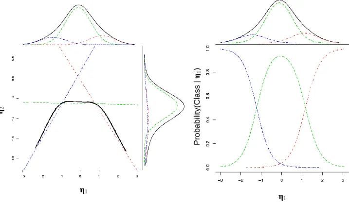
Figure 1 offers a visual representation of this process with two latent variables, where
a SEMM with 3 classes is used to approximate a quadratic shaped function. In the left panel
of Figure 1 the expected value of 𝜂2 is represented by a solid black line and the within class
linear functions are represented by dashed lines. The right panel of Figure 1 shows the
probability weights that are applied to the within-class linear functions to create the nonlinear
aggregate function.
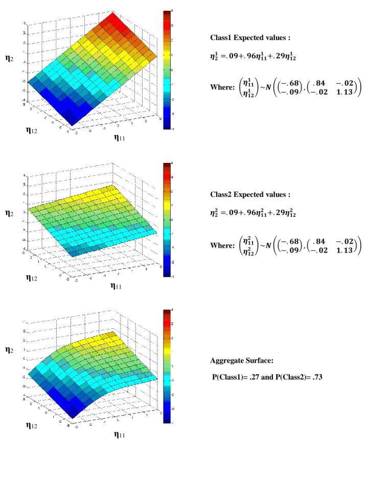
To model interaction effects, this approach can also include two latent exogenous
variables that influence a latent endogenous variable. In this case the within-class functions
would be represented by planes instead of lines and the weighting of the planes by their class
14
of the three dimensional case, where a 2-class SEMM is fit to a nonlinear surface, can be
seen in Figure 2. The top two panels are the within-class planes, while the bottom panel
contains the nonlinear surface of the overall expected values for 𝜂2 across classes.
The advantage of the SEMM approach is that it makes very weak assumptions
regarding the distributions of the latent and observed variables, specifically it assumes that
the distribution can be approximated by a finite mixture of normal distributions. Another
advantage of the SEMM approach is that it does not assume a specific functional form of the
latent regression surface, instead it assumes that the form of the surface can be approximated
by a mixture of planes. A disadvantage of not specifying a functional form is that the method
cannot provide a specific estimate for the interaction parameter to test for significance, which
can be obtained with the parametric methods. Because the model requires fewer assumptions
it is better able to capture the nuances of the data, however, this flexibility may result in
increased sampling variability. To assess these potential advantages and disadvantages, the
semiparametric approach should be investigated to see how well it approximates the true
relationships among the latent variables.
Previous Studies Using Structural Equation Mixture Models
Simulation studies by Bauer (2005) and by Bauer, Mathiowetz and Gottfredson
(2010) found support for use of the SEMM approach to detect nonlinear relationships
between two latent variables across a variety of conditions. Bauer (2005) examined a
quadratic trend and used plots of averaged estimates from the SEMM approach to show that
the approach produced unbiased estimates relative to the true model. The plots also showed
how the bias in the estimates decreases when additional classes are used and how the
15
Similarly Bauer, Mathiowetz and Gottfredson (2010) found that the estimates from
the SEMM approach had low bias when plotted against the predicted values from the true
data generation model. Further, SEMM estimates were found to have less bias than estimates
obtained from loess regression on factor scores estimates. This lower bias was found across
sample size (n=250, 500, 1000), number of indicators (3 or 6) and size of the quadratic effect
(-.35 or -.5). The estimates from the SEMM approach tended to be less efficient than those
obtained when using a loess procedure with factor scores. Further simulation work examined
the performance of the SEMM approach when applied to data generated from a linear model
to test whether this approach would produce spurious nonlinear curve estimates. Results
showed that the SEMM approach could recover a linear trend even when SEMMs with more
than one class were found to fit best. Overall, the results suggested that SEMM approach
could closely approximate the true model.
Although neither Bauer (2005), nor Bauer, Mathiowetz and Gottfredson (2010)
examined latent variable interactions, the successful approximation of the relationship
between two variables supports the exploration of the SEMM approach for evaluating latent
variable interactions. The challenge for the SEMM approach will be to go from lines
approximating a curve to planes approximating a nonlinear surface. The SEMM approach
may require more planes to approximate a surface than were needed when approximating a
curve with lines. If the sample size is not large enough for SEMMs with more classes to
converge, the SEMM approach may not be able to fit a model complex enough to closely
approximate the surface. Similarly, if the data in a given sample is not located in the
16
more than one class. These potential challenges suggest the need to study the performance of
the SEMM approach as a method to estimate latent variable interactions.
Current study
This study proposes to use simulation methodology to examine the potential utility of
the SEMM approach to estimate latent variable interactions. Based on the results from Bauer,
Mathiowetz and Gottfredson (2010), it is hypothesized that the SEMM approach will not
detect an interaction when one is not present. Therefore a main effects only condition was
included to test this hypothesis. In addition to the main effects model, a nonlinear model with
no interaction was included to test the hypothesis that the SEMM approach can distinguish
between a nonlinear surface with and without an interaction. Besides the models with no
interactions, two models with interactions were included to test if the SEMM approach can
approximate a variety of interactions. Specifically, it is hypothesized that because the SEMM
approach does not specify a functional form for the relationships among the latent variables,
the approach should be able to approximate both bilinear and nonlinear interactions.
The performance of the SEMM will be judged in terms of its accuracy in recovering
the true model regression surface. In the main effects model, an SEMM with one class would
correctly identify that the data were generated from a plane. For the nonlinear model, the
SEMM approach should estimate a model with more than one class to approximate the
nonlinearity of the data, but plots of the estimated surface from the SEMM approach should
show that the additional classes approximate a nonlinear surface rather than an interaction
surface. In contrast to the nonlinear data generation condition, the SEMM approach should
17
conditions. As with the nonlinear condition, plots of the estimated values from the SEMM
approach should reveal an interaction surface rather than a nonlinear surface.
There are several factors that may influence the performance of the SEMM approach.
For example, previous studies have found the SEMM approach may require additional
classes to accommodate non-normally distributed latent exogenous variables or latent
endogenous disturbances (Bauer & Curran, 2003). However, based on the findings that
models with additional classes did not lead to a spurious nonlinear relationship in previous
studies of the SEMM approach, it is hypothesized that the SEMM approach should perform
equally well at detecting latent variable interactions with both normal and non-normally
distributed latent variables. To evaluate this hypothesis, each data generation model (main
effects, nonlinear, bilinear interaction, nonlinear interaction) included one variation with
normally distributed latent variables and another with non-normally distributed latent
variables.
In addition to examining the performance of the SEMM approach with non-normal
latent variable distributions, it is important to evaluate its performance in finite sample sizes.
Previous studies of SEMMs have found that larger sample sizes can be associated with
SEMMs with more classes being selected as best fitting models (Lubke & Neale, 2006).
Because the SEMM approach uses multiple linear surfaces to approximate a nonlinear
surface, it may require more data to fit a sufficient number of classes to capture the
underlying relationships among the data. The SEMM approach should therefore be better at
detecting interactions with larger sample sizes. To evaluate this issue, this study examined
18
Lastly, the correlation between the exogenous factors will influence the joint
distribution of the data such that correlated exogenous factors that are normal or unimodally
distributed will have more observations clustered on the diagonal. This clustering will result
in a lower probability of having observations in the four extremes of the joint distribution.
Based on the findings of McClelland and Judd (1993), the more correlated the latent
exogenous variables are the less information there will be to detect an interaction. Thus, it
was hypothesized that the performance of the SEMM approach should be worse when the
Chapter 2
METHOD
To evaluate the utility of the SEMM approach to estimating latent variable
interactions a simulation study with a 3 X 2 X 2 X 4 design was used. The design included
three sample sizes, 250, 500 and 1000, as well as two exogenous latent variable distributions,
normal and χ²(6), and the exogenous latent variables were either uncorrelated or correlated
.71. Lastly, the design included four data generating models: main effects, nonlinear, bilinear
interaction and nonlinear interaction.
Population models
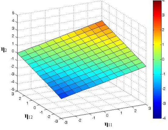
For the main effects model a population structural equation model was parameterized
as
𝐸(𝜂2 𝜂11, 𝜂12 = 0.4𝜂11 + 0.4𝜂12 (17)
Where 𝜂11 and 𝜂12 represent the latent exogenous variables and 𝐸(𝜂2 𝜂11, 𝜂12 is the
expected value of 𝜂2 given 𝜂11 and 𝜂12. A plot of the expected values of this model can be seen in Figure 3.
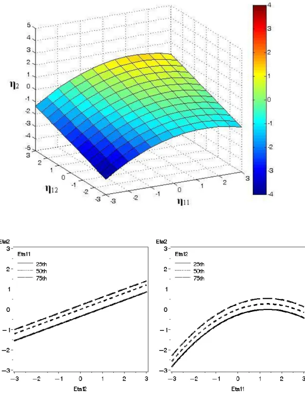
The nonlinear model was generated using a population structural equation model
parameterized as
𝐸(𝜂2 𝜂11, 𝜂12 = 0.4𝜂11 + 0.4𝜂12− 0.15𝜂112 (18)
A plot of the expected values of this model can be seen in the top plot of Figure 4. The
bottom two plots in Figure 4 contain the simple slopes of the endogenous factor for each
20
percentiles. The nonlinear effect for the nonlinear model was chosen to be a value that
represents approximately a 5% increase in R-square when it is included in the model.
The bilinear interaction model followed a population generating function of
𝐸(𝜂2 𝜂11, 𝜂12 = 0.4𝜂11 + 0.4𝜂12+ 0.2𝜂11𝜂12 (19)
The interaction effect was also chosen to be a value that represents approximately a 5%
increase in R-square when it is included in the model. Figure 5 shows several plots of the
expected values of the bilinear interaction model. The top plot represents the overall function
while the bottom two plots contain the simple slopes of the endogenous factor for each
exogenous factor while holding the other exogenous factor constant at the 25th, 50th and 75th percentiles.
For the second interaction model, the nonlinear interaction was generated as
𝐸(𝜂2 𝜂11, 𝜂12 = 1.16 − exp(−0.5𝜂11 − 0.25𝜂12− 0.1𝜂11𝜂12) (20)
As with the nonlinear and bilinear interactions models, the interaction effect for the nonlinear
interaction model was also chosen to be a value that represents approximately a 5% increase
in R-square when it is included in the model. Figure 6 contains a plot of the expected values
for the nonlinear interaction model as well as the simple slope plots for each exogenous
factor.
The population parameter values for the main effects and bilinear interaction models
come from Marsh, Wen and Hau (2004). These parameters were selected in order to have
similar parameters to those used in previous simulation studies of approaches to detect latent
variable interactions. The nonlinear interaction model population parameters were chosen so
21
interaction models. To my knowledge, nonlinear interactions have not previously been
examined in the literature.
Data Generation
For all three models, the latent exogenous variables η11 and η12 were standardized variables that had either a normal distribution or a skewed distribution, χ²(6), rescaled to
M=0 and SD=1. The influence of correlated latent exogenous variables was examined by
generating 𝜂11 and 𝜂12 to either have no correlation or a correlation of .71. For each
population model the total variance of 𝜂2 was set to approximately 1 by adding normally
distributed errors with M=0 and SD=.71 to each of the values computed from Equation 16,
17, 18 or 19. Across all conditions, the latent variables, 𝜂11, 𝜂12 and 𝜂2, each had three
indicators. For simplicity, in the data generating model the factor loadings for the indicators
were 1 for all indicators, and their communalities were .75. The indicators were formed by
adding normally distributed errors to the latent factor scores. For each data generation
condition 250 data sets were generated.
Model Fitting
SEMMs were fit using Mplus Version 5.0 (Muthén & Muthén, 2007). For each data
set a one-class model and then models with increasing number of classes were fit for up to 5
classes or until model fit as indexed by the BIC no longer improved. To reduce computation
time and reduce the likelihood of local solutions start values were obtained by fitting mixture
models to large data sets (500,000 observations) generated for each condition. Mixture
models with two, three, four and five classes were fit using 500 random starts with the 10 of
the initial stage iterations taken to the final stage optimization. The start values obtained from
22
which used 10 random starts with the two of the initial stage iterations taken to the final stage
optimization. The model with the number of classes with the lowest BIC was selected as the
model of best fit for each data set. The BIC was selected because it is a commonly used
index for class selection. The results presented are for all 250 replications with the exception
of two replications that that did not converge in the nonlinear interaction condition with
normally distributed and uncorrelated data at both the 500 and 1000 sample sizes.
Evaluating Model Performance
To evaluate the performance of the SEMM approach I calculated the discrepancy
between the estimated regression surface obtained from the best fitting SEMM and the
regression surface of the true data generating model. Based on Equation 2.37 in Kendall and
Stuart (1969, Vol. 1, p. 51) the expected value of the squared difference, or mean-squared
error (MSE) for a given replication r is
𝑀𝑆𝐸𝑟 = 𝐸 𝑔𝑆𝐸𝑀𝑀𝑟 𝜼1 − 𝑔𝑇𝑟𝑢𝑒 𝜼1 2 = 𝑔𝑆𝐸𝑀𝑀𝑟 𝜼1 − 𝑔𝑇𝑟𝑢𝑒 𝜼1
2
𝑓 𝜼1 𝑑𝜼1 (21)
Where 𝜼1 represents the values for the exogenous variables, 𝑔𝑆𝐸𝑀𝑀𝑟 𝜼1 the
predicted value of 𝜂2 from the SEMM approach and 𝑔𝑇𝑟𝑢𝑒 𝜼1 the predicted value of 𝜂2
from the true data generation model. The Probability Density Function (PDF) of 𝜼1 is
designated as 𝑓 𝜼1 . In this simulation, the PDF is either multivariate normal or a
standardized multivariate chi-square χ²(6) distribution. Note that the discrepancy is weighted
by the PDF of the predictor such that values which occur more often are given a greater
weight than those that are less likely to be observed.
To enable MSE calculations for each replication, the integral in Equation 21 was
approximated using Monte Carlo numerical integration. First, 10,000 values for 𝜂11 and 𝜂12
23
observed data sets. Then the 10,000 simulated values were used to calculate predicted values
for the latent endogenous outcome from the SEMM (i.e. 𝑔𝑆𝐸𝑀𝑀𝑟 𝜼1 ) using Equation 15, as
well as the expected value for the true data generation model (i.e. 𝑔𝑇𝑟𝑢𝑒 𝜼1 , see Equation
17, 18, 19 and 20). By taking the squared difference of these estimates and calculating their
sum over the simulated values an estimate of MSE was obtained for each replication. This
MSE calculation for a given replication, r, can be expressed as
𝑀𝑆 𝐸𝑟 = 𝑔𝑆𝐸𝑀𝑀𝑟 𝜼1 − 𝑔𝑇𝑟𝑢𝑒𝑟 𝜼1
2 10000
𝑚=1 /10000 (22)
An overall MSE for each condition of the simulation can then be calculated as
𝑀𝑆 𝐸𝑇 = 250 𝑀𝑆 𝐸𝑟
𝑟=1 /250 (23)
The root mean squared error (RMSE) is obtained by taking the square root of the MSE
estimate. The MSE and RMSE were used to numerically evaluate overall model fit, with
lower values representing better fit.
The overall MSE was also decomposed into components reflecting bias and sampling
variance. A description of this alternative formula can be found in Section 17.30 of Kendall
and Stuart (1969, Vol. 2, p. 21), and the equation can be expressed as
𝑀𝑆𝐸𝑇 = 𝐵2 + 𝑉 (24)
Where 𝐵2 represents the squared bias component and 𝑉 represents the variance of the
estimates.
For the current case, the general form of 𝐵2 is expressed as
𝐵2 = [𝑔
𝑆𝐸𝑀𝑀 𝜼1 −𝑔𝑇𝑟𝑢𝑒 𝜼1 ]2𝑓 𝜼1 𝑑𝜼1 (25)
Where 𝑔𝑇𝑟𝑢𝑒 𝜼1 is the predicted value of 𝜂2 obtained from the true function and 𝑔 𝑆𝐸𝑀𝑀 𝜼1
is the average predicted value of 𝜂2 obtained from the SEMM at a given value of 𝜼1 across
24
𝑔 𝑆𝐸𝑀𝑀 𝜼1 = 250𝑔𝑆𝐸𝑀𝑀𝑟 𝜼1 /250
𝑟 (26)
To calculate squared bias in the current study, Equation 25 was approximated using Monte
Carlo numerical integration using the following equation
𝐵2 ≈ [𝑔
𝑆𝐸𝑀𝑀 𝜼1 − 𝑔𝑇𝑟𝑢𝑒 𝜼1 ]2 10000
𝑚 =1 /10000 (27)
Besides squared bias, the variance of the SEMM approach was also calculated. The
equation for variance (𝑉) is
𝑉 = [𝑔𝑆𝐸𝑀𝑀𝑟 𝜼1 − 𝑔 𝑆𝐸𝑀𝑀 𝜼1 ]2𝑓 𝜼1 𝑑𝜼1 (28)
Similar to the squared bias component, Monte Carlo numerical integration was used as an
approximation for Equation 28. The numerical integration formula for 𝑉 can be given as
𝑉 ≈ 10000𝑚 =1 [𝑔𝑆𝐸𝑀𝑀𝑟 𝜼1 − 𝑔 𝑆𝐸𝑀𝑀 𝜼1 ]2/10000 (29)
By comparing 𝑀𝑆𝐸𝑇, 𝐵2 and 𝑉 across conditions the relative performance of the
SEMM approach can be evaluated. Because the population variance of 𝜂2 was set to be
approximately 1 during data generation, simply taking the square root of 𝑀𝑆𝐸𝑇, 𝐵2 and 𝑉
puts these estimates into SD units of 𝜂2. Thus the magnitude of the bias and standard error
(𝑉1/2) can be judged relative to the overall standard deviation of the outcome.
In addition to evaluating the performance of the SEMM approach numerically, it was
also evaluated visually. One way to visually evaluate the SEMM approach is to create a
surface plot of the bias. This plot can be obtained by selecting exogenous factor observations
that span the grid of potential observations, in this case, observations ranging from –3 to 3 for
𝜂11 and 𝜂12. By using this grid of observations to generate predicted values from the SEMM
approach and the data generating model, plots of the bias at each point were used to create a
bias surface. This estimated surface was used to evaluate where the SEMM approach is
25
In addition to bias surface plots, simple slope plots similar to those found in Figures
4, 5 and 6 were constructed to visually assess the SEMM approach. These plots show the
Chapter 3
RESULTS
The results will be presented as follows: first, the information on SEMM
convergence rates and class selection will be presented, then the results for the performance
of the SEMM approach in terms of the numerical indices and plots will be presented by data
generating model (e.g. main effect, nonlinear, etc.). The results measuring the numerical
performance of the SEMM, will include estimates of bias, standard deviation and RMSE, for
all conditions. The recovery of the true surface will be presented using three-dimensional
estimated average surface plots and bias surface plots for a subset of the conditions.
Similarly, a subset of simple slope plots will be presented to show the recovery of the true
surface conditional on levels of the exogenous variables. An appendix will include plots for
additional conditions. After presenting the performance results by data generating model, a
summary of the results across data generation conditions will be provided.
Convergence and BIC Class Selection
For most of the conditions the SEMMs converged for all replications. Appendix A
contains the percent of replications that converged to proper solutions. When the sample
size was 250 and the SEMM had 4 or 5 classes the convergence rates were lower, but they
were still typically greater than 70 percent. Information on the convergence rates and how
frequently a given number of classes was selected as best by the Bayesian Information
27
rates were found in the correlated conditions and higher convergence rates were found in the
conditions with skewed data.
Main Effects Model
A main effects model was included to evaluate if spurious interactions would be
detected by the SEMM approach when no interaction or nonlinearity was present. As
hypothesized, the SEMM approach did not find any nonlinearity when the data were
generated from a main effects model. The numerical performance of the SEMM approach for
the main effects data generation model can be seen in Table 1. The estimates for bias,
standard deviation and RMSE are given for the number of classes most frequently selected as
best by the BIC. The results suggest that when there is no interaction or nonlinearity in the
regression surface, the SEMM approach estimated a one-class model as best, as long as the
data is normally distributed. This provides de facto support for the hypothesis that the SEMM
approach would not detect spurious interaction. However, when the data was generated to be
skewed, BIC selected SEMMs with more than one class as best. The additional classes in the
skewed condition only increase the overall bias of the estimated surface a trivial amount,
suggesting that the estimated surface is very similar to the data generating model. The
increase in RMSE for the skewed data conditions is associated with the increase in
variability, as indicated by the standard deviation values.
To demonstrate that this increase in variability may come from the additional classes,
values for RMSE, bias and standard deviation for the one-class SEMM results can be seen in
Table 2. The results in Table 2 reveals that the standard deviation values in the skewed data
conditions are almost identical to the values for the normally distributed data in Table 1.
28
distributed data in Table 1. The results in Table 1 and Table 2 suggest that having skewed
data may result in the BIC selecting SEMMs with additional classes as best fitting the data,
however these additional classes do not seem to dramatically influence the bias, instead the
additional classes increase the variability of the surfaces estimated by the SEMM approach.
Besides holding the number of classes constant, one can examine bias by examining
the estimated surface plots directly. Surface plots of the predicted values from the SEMM
approach were generated for observations ranging from –3 to 3 for 𝜂11and 𝜂12. Figure 7
shows the SEMM estimated average surface plots for all three sample sizes for the main
effects conditions where the data was generated to be skewed and either uncorrelated (left) or
correlated (right). The main effects plots in Figure 7 do not appear to have any nonlinear
features and are therefore very similar to the surface that was used to generate the data shown
in Figure 3. These results suggest that even when a model with more than one class is
selected as best the estimated surface will not show spurious interactions when the data are
generated from a main effects model.
Nonlinear Model
Besides the main effects condition, a second model with no interaction was included
to assess whether the SEMM approach would suggest the presence of an interaction when the
data was generated from a nonlinear function without an interaction. Table 3 contains the
numerical performance of the SEMM approach for the nonlinear data generation model for
the number of classes most frequently selected as best by the BIC. The results in Table 3
indicate that the BIC did select an SEMM with multiple classes to approximate a nonlinear
surface with few exceptions. Specifically, a one-class SEMM was found to fit best according
29
the conditions where more than one class was selected as best, the RMSE and bias were
substantially lower than the conditions where the one-class SEMM was found to fit best.
The results in Table 3 show that the standard deviation tended to get lower as sample
size increased, with the exception of when the data was generated to be normal and where the
sample size went from 500 to 1000. It is possible that going from a one-class model to a
two-class model led to an increase in the variability of the estimated surfaces. To examine this
possibility Table 4 contains the RMSE, bias and standard deviation results for the SEMM
approach for the two-class solutions for all the nonlinear model conditions. Table 4 shows
that when number of classes is held constant, the standard deviation decreases as the sample
size increases. In addition to clarifying the relationship between variability and sample size,
Table 4 shows the tendency for all indices of performance to be higher for data generated to
be skewed relative to normally generated data. This does not fit with the hypothesis that the
SEMM approach would perform equally well with normal and non-normally distributed data.
Further examination of Table 4 shows that the bias is significantly lower for the
two-class results compared to the bias in Table 3 where a one-two-class SEMM was selected by the
BIC as best. This suggests that a model with additional classes would more closely
approximate the true data generation model. This closer approximation of the true surface is
accompanied by an increase in standard deviation, although the increase in variability does
not prevent the overall measure of performance, RMSE, from being lower for the two-class
SEMM approximation in these conditions. Table 4 also shows that bias decreases slightly
within a condition as sample size increases. This suggests that sample size does not influence
30
The selection of a one-class SEMM as best did not support the hypothesis that the
SEMM would estimate additional classes to approximate the nonlinearity of the data, but this
only occurred in conditions where the information from the data was sparse. However, the
conditions that do estimate additional classes support that hypothesis. To further evaluate
whether the additional classes were approximating the nonlinearity and not a spurious
interaction, plots of the estimated surface from the SEMM approach were examined. Figure 8
contains the estimated surface plots for several nonlinear data generation conditions.
Specifically, Figure 8 contains the estimated average surface plots for the BIC best class
SEMM for the sample sizes of 250 (top), 500 (middle) and 1000 (bottom), when the data was
generated to be skewed and either uncorrelated (left) or correlated (right).1 Overall, the plots show a similar shape to the surface used to generate the data (see Figure 4) and do not appear
to show any interaction between the two exogenous variables. These results suggest that
when the data is generated from a nonlinear model, the SEMM will detect the nonlinearity
and not detect spurious interactions. Additional surface plots for the nonlinear model can be
seen in Appendix B.
In addition to the estimated surface plots, the performance of the SEMM approach
was also evaluated using simple slope plots. Figure 9 contains the simple regression line
plots for the nonlinear data generation condition with skewed and correlated data. The black
lines in the plot represent the simple regression lines for the data generation model, while the
blue lines represent the SEMM results. The top plots show the two-class SEMM results for a
sample size of 250, the middle plots show the two-class SEMM results for a sample size of
500 and the bottom plots show the four-class SEMM results for a sample size of 1000. There
1 There were no observations for values of 𝜂
11 and 𝜂12 less than -1.73 in the skewed distribution. The results
31
are no results plotted for values of 𝜂11 and 𝜂12 less than -1.73 because those values were not
observed in the skewed distribution.
Across the sample sizes, Figure 9 shows that the estimates appear to closely follow
the data generating model for the linear relationship between 𝜂12 and 𝜂2. The simple slope
plots provide important information because they have relatively parallel lines, suggesting
that there is no interaction between 𝜂11 and 𝜂12, and simply a nonlinear relationship between
𝜂11 and 𝜂2. These simple regression line plots also show that the while SEMM provides a
relatively unbiased approximation for the linear relationship between 𝜂12 and 𝜂2, the
approximation for the nonlinear relationship between 𝜂11 and 𝜂2 tends to have more bias,
especially for the parts of the distribution that have fewer observations (e.g. 𝜂11 and 𝜂12 less
than -1.26 or greater than 1.90). These plots suggest that the SEMM approach will better
approximate linear relationships and will have a better approximation of nonlinear surfaces
where more data is observed.
Bilinear Interaction Model
In addition to the models with no interactions, two models with interactions, bilinear
and nonlinear, were included to assess the performance of the SEMM approach for different
interaction forms. The results for the numerical performance of the SEMM approach for the
bilinear interaction model can be seen in Table 5. For most of the conditions, as
hypothesized, the BIC selected an SEMM with more than one class as best. Typically either a
two-class or three-class SEMM was selected most frequently by the BIC. One exception to
this pattern was the condition with normally distributed and correlated data where the BIC
32
small sample sizes and correlated data researchers may find that the BIC will select a
one-class solution as best even though the data were not generated from a main effects model.
Examining the numerical indices of performance in Table 5 reveals several trends.
First, the RMSE results in Table 5 show that when the data was generated to be skewed or
correlated, the RMSE tends to be slightly higher relative to the uncorrelated or normally
distributed data. This trend seems to come from a slight increase in bias as well as increased
surface variability, as indicated by standard deviation. The results for correlated versus
uncorrelated conditions support the hypothesis that the SEMM approach would perform
better for uncorrelated data. However, the trend for skewed versus normal data does not
support the hypothesis that the SEMM approach would perform equally well regardless of
the distribution of the latent predictors. Examination of the difference in RMSE for skewed
versus normally distributed data does suggest that it may be small relative to the influence of
other variables (e.g. sample size). Furthermore, the difference in RMSE may not be
concerning because it was not associated with spurious interactions or exaggerated
nonlinearity (see Appendix B).
In addition to the trends for the latent variable distributions and the correlation of the
data, Table 5 also shows a sample size trend. As with the nonlinear model, surface variability
tends to decrease with higher sample sizes resulting in lower RMSE as sample size increases.
However, this effect is influenced by the number of classes found to be best, such that in the
condition where the data were generated to be normal and correlated going from a sample
size of 250 to 500 also involves going from one to two classes as best which results in
increased surface variability. In the conditions with normally distributed, uncorrelated data,
33
size. This condition shows that similar to the nonlinear data generating model, there is
relatively little change in bias as sample size increases, and therefore any decrease in RMSE
is because of the decrease in surface variability.
To examine the trends in RMSE, bias and standard deviation without the influence of
changing number of classes, Table 6 contains the results for the two-class SEMMs for all of
the bilinear interaction conditions. Table 6 clearly shows that as sample size increases,
surface variability and RMSE decrease. This supports the hypothesis that the SEMM
approach would perform better with larger sample sizes. Table 6 also shows that bias either
remains relatively stable or increases slightly (e.g. increases of .002 or .003) across sample
sizes, indicating that that sample size primarily influences surface variability.
As with Table 5, RMSE tends to be higher for correlated or skewed data relative to
normal or uncorrelated data. However, when controlling for number of classes, bias is
relatively equal for both correlated and uncorrelated data, but higher for skewed relative to
normally distributed data. These bias results do not support the hypothesis that the SEMM
approach would perform worse for the correlated data or the hypothesis that the SEMM
approach would perform equally well for skewed and normally distributed exogenous
variables.
As with the main effects and nonlinear conditions we can visually assess the
performance of the SEMM approach using surface plots of the predicted values from the
SEMM approach. Because the surfaces in the interactions are more complicated than the
previous conditions, surface plots of the bias will also be presented for the interaction
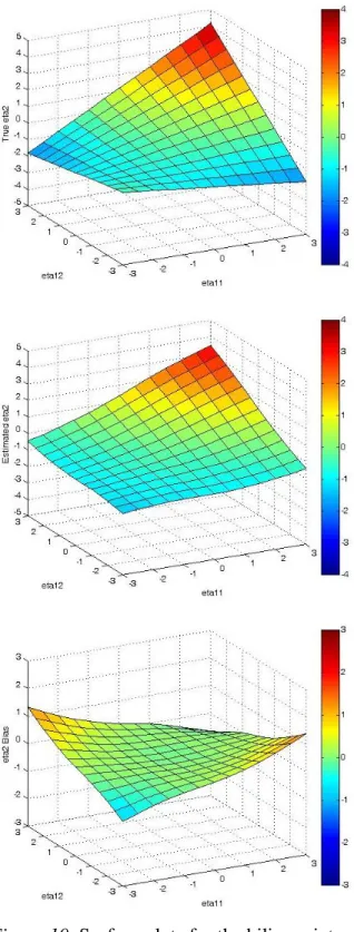
conditions. To show how the bias surface plots where constructed, Figure 10 contains the
34
SEMM (middle panel) and estimated bias surface (bottom panel) for the bilinear interaction
condition with normally distributed, uncorrelated data with a sample size of 1000.2 The results for the sample size of 1000 should fairly represent this condition because the bias was
approximately equal for all sample sizes in this condition. The overall shape of the estimated
surface is very similar to the surface used to generate the data. As shown in the bias surface
plot, the difference between the surfaces appears at the extremes of the exogenous
distributions. This suggests that the SEMM is performing best where the data is more
frequently observed, which fits with the performance of SEMM in other studies as well as
with our hypothesis that the SEMM would perform best where there was more observed data.
To show that the average bias plot does reflect how a given replication would
perform, the Figure 11 shows the true surface (top), estimated surface (middle) and the
discrepancy surface (bottom) for one replication‟s results for the same conditions as those
shown in Figure 10. Similar to the results for the average surface plot, the estimated surface
plot for one replication also has an overall shape very similar to the surface used to generate
the data, although it is less smooth than the average estimated surface. The discrepancy plot
in Figure11 shows more bias in the extremes as well as a less smooth surface in the center of
the joint exogenous distribution. Together the plots in Figure 10 and 11 indicate that the
average estimated surfaces will appear smoother than the results of a given replication, but
the overall shape should reflect the performance of a given replication.
An example of the effect of normal versus skewed data can be seen in Figure 12
which contains the estimated average surface and average bias surface plots for the results of
the two-class SEMM fit to data from the bilinear interaction model with uncorrelated data at
2
35
a sample size of 250. The plots on the left represent the results for the normally distributed
data, while the plots on the right are from skewed data. The estimated surface plots (top)
show that the normally distributed data has a smoother approximation of the data generating
surface (see Figure 5). The average bias surface plots (bottom) show the bias to be greater for
the skewed data condition for the parts of the distribution that have fewer or no observations
(e.g. when 𝜂11and 𝜂12 are less than -1.26 or less than -1.73), and less bias where the skewed
data has more observations than the normal data (e.g. 𝜂11and 𝜂12 greater than 1.68). These
plots fit with the bias results in Table 5. For the normally distributed condition the average
bias was .0698, whereas in the skewed condition the bias was .1042. Taken together the
numerical indices show the overall size of the bias, while the plots show where the bias is
occurring. Although the numerical indices of bias do not support the hypothesis that the
SEMM approach would perform equally well regardless of the latent variable distributions,
the plots do support the hypothesis that the SEMM approach will perform better where there
are more observations.
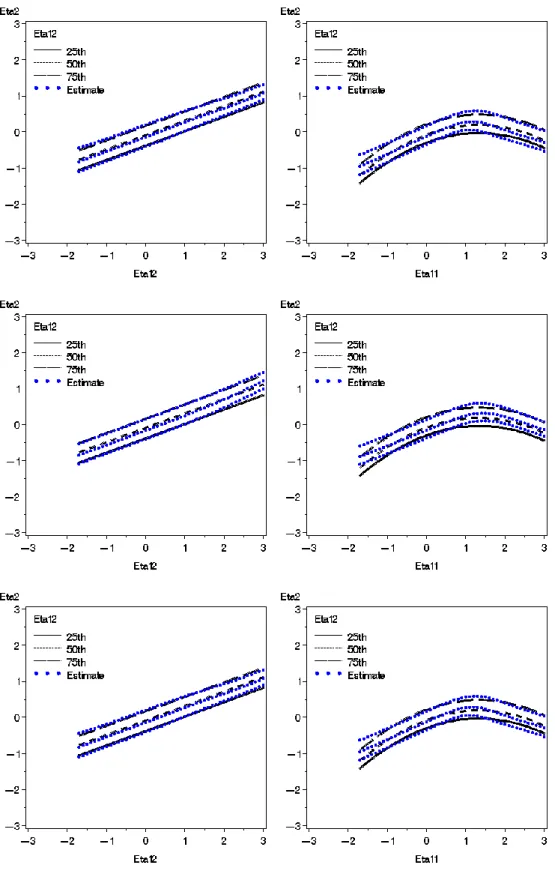
In addition to examining the numerical indices, simple slope plots can also reveal the
effects of having correlated exogenous variables. Figure 13 contains some simple slope plots
from the bilinear interaction data generating model with normally distributed data at a sample
size of 1000. The top plots show the two-class SEMM results for uncorrelated exogenous
variables while the bottom plots show the two-class SEMM results for correlated exogenous
variables. As the bias is relatively equal across sample sizes, these plots should reflect the
pattern of results across sample sizes. For both correlated and uncorrelated data the SEMM
approach tends to better approximate the true values where more data is observed (e.g. values