ADVANCES IN DATA-DRIVEN RESEARCH METHODOLOGY FOR PRECISION PUBLIC HEALTH
Michael T. Lawson
A dissertation submitted to the faculty of the University of North Carolina at Chapel Hill in partial fulfillment of the requirements for the degree of Doctor of Philosophy in the Department
of Biostatistics in the Gillings School of Global Public Health.
Chapel Hill 2019
Approved by: Michael R. Kosorok Eric B. Bair
Michael I. Love
ABSTRACT
Michael T. Lawson: Advances in Data-driven Research Methodology for Precision Public Health (Under the direction of Michael R. Kosorok)
The rise of precision medicine has ushered in manifold opportunities and challenges, many of them linked. For instance: precision medicine offers an avenue to revisit assumption-rich, knowledge-driven research practices, but requires careful and creative thinking to replace them. In this manuscript, we turn our attention to three such areas of interest: subgroup determina-tion, modeling of dynamical systems, and accounting for measurement error. In each case, we construct a statistical and machine learning framework for the problem at hand, develop method-ology to address it, and present theoretical and numerical justifications for the methodmethod-ology.
ACKNOWLEDGEMENTS
TABLE OF CONTENTS
LIST OF TABLES . . . ix
LIST OF FIGURES . . . x
LIST OF ABBREVIATIONS . . . xv
CHAPTER 1: INTRODUCTION . . . 1
CHAPTER 2: PRECISION MEDICINE SUBGROUP ANALYSIS . . . 3
2.1 Introduction . . . 3
2.2 Methods . . . 5
2.3 Results. . . 9
2.4 Discussion . . . 11
2.5 Measures . . . 14
2.5.1 Measurement Methodology . . . 14
2.5.2 Outcome Variables . . . 16
2.5.2.1 HbA1c univariate outcome . . . 16
2.5.2.2 QoL univariate outcome . . . 17
2.5.2.3 BMIz univariate outcome . . . 17
2.5.2.4 Composite Outcome . . . 18
2.6 Properties of composite outcome . . . 19
2.6.1 Numerical Experiments . . . 21
2.6.1.1 Experiment in Simple Conditions . . . 23
2.6.1.2 Experiment in Trial-Like Conditions . . . 24
2.7 Sensitivity Analyses . . . 31
2.8 Outcome weighted learning (OWL) . . . 35
2.9 Imputation Bootstrapping Procedure. . . 35
CHAPTER 3: VOLATILITY LEARNING IN DYNAMICAL SYSTEMS . . . 38
3.1 Introduction . . . 38
3.2 Methods . . . 40
3.2.1 Notation . . . 40
3.2.2 Proposed Model . . . 41
3.2.3 Estimating the Process Mean . . . 42
3.2.4 Estimating the Process Volatility . . . 43
3.3 Theoretical Properties . . . 47
3.4 Simulations . . . 52
3.4.1 Variable selection in additive ODEs . . . 53
3.5 Clinical Application . . . 54
3.5.1 CCAT study and data . . . 54
3.5.2 Application to CCAT study . . . 56
3.6 Discussion . . . 57
CHAPTER 4: MEASUREMENT INFLUENCE DIAGNOSTICS . . . 59
4.1 Introduction . . . 59
4.2 General Framework . . . 60
4.3 Method . . . 61
4.4 Numerical Experiments . . . 63
4.4.1 Regression Setting . . . 63
4.4.1.1 Impact of Modeling Uncertainty . . . 71
4.4.2 Precision Medicine Setting . . . 79
4.5.1 Forest Fires . . . 85
4.5.2 Water Source Microbial Content . . . 86
4.6 Discussion . . . 88
CHAPTER 5: DISCUSSION AND FUTURE RESEARCH . . . 91
APPENDIX A: TECHNICAL DETAILS FOR CHAPTER 3 . . . 95
A.1 Proofs . . . 95
A.1.1 Notation . . . 95
A.1.2 Proof of Theorem 3.1 . . . 96
A.1.3 Proof of Theorem 3.2 . . . 98
LIST OF TABLES
2.1 Estimated Value (Bootstrap 95% Confidence Interval) of RLT Imputed ITR
by Outcome Variable . . . 9 2.2 Subgroup Recovery Sensitivity and Specificity by Treatment Effect (Simple
Experiment, Synergistic Setting) . . . 28 2.3 Treatment Effect MSE by True Treatment Effect (Simple Experiment,
Syn-ergistic Setting) . . . 28 2.4 Treatment Effect MSE by True Treatment Effect (Simple Experiment,
An-tagonistic Setting) . . . 29 2.5 Subgroup Recovery Sensitivity and Specificity by Method and Treatment
Ef-fect (Trial-Like Conditions, Synergistic Setting) . . . 30 2.6 Treatment Effect MSE by True Treatment Effect (Trial-Like Conditions,
Syn-ergistic Setting) . . . 30 2.7 Treatment Effect MSE by True Treatment Effect (Trial-Like Conditions,
An-tagonistic Setting) . . . 31 2.8 Estimated Value (Bootstrap 95% Confidence Interval) of ITR by Method, Dataset,
and Outcome Variable . . . 32
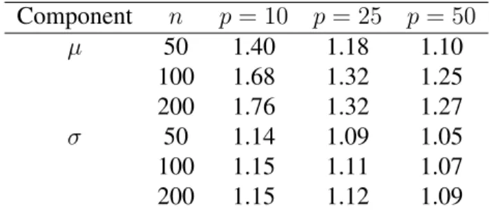
3.1 Average sens+spec forSˆµandSˆσ acrossN = 100independent
simula-tion runs and various values ofnandp. . . 54
4.1 Percentage of observations with|rank(∆i`)−rank(∆i,`−1)|<10, by value
ofγ`. . . 79 4.2 The∆values, area burned (ha), X and Y coordinates within the Montesinho
park area (both ordinal from 1 to 9), month, FFMC index, ISI index, temper-ature in degrees Celsius, relative humidity in %, and wind speed in km/h of the fifteen most measurement influential forest fires in the data of Cortez and Morais (2007).∆values were obtained using the RF model withΨ(P) =
ˆ
Y andΓ(Y)lying symmetrically about the raw burned areaY˜, clipped be-low at zero, and then log-transformed before analysis as the outcome
LIST OF FIGURES
2.1 (A-C). RLT-predicted values ofRby true treatment effect, intervention status, and true split-ting variableXfor the simple numerical experiment of Section 2.6.1.1, synergistic setting. The true treatment effects forR1andR2are set toδ1=δ2= 1,3,10in A, B, and C, re-spectively. (D-F). Differences in predicted composite rewardRbetween intervention and control by true treatment effect, RLT ITR assignment, and true splitting variableX, as well as the true treatment effect forR, for the same numerical experiment. ITR=2 denotes the true treatment effect forR. The true treatment effects forR1andR2are set toδ1=δ2=
1,3,10in D, E, and F, respectively. . . 25 2.2 (A-C). RLT-predicted values ofRby true treatment effect, intervention status, and true
split-ting variableXfor the simple numerical experiment of Section 2.6.1.1, antagonistic setting. The true treatment effects forR1andR2are set toδ1=δ2= 1,3,10in A, B, and C, re-spectively. (D-F). Differences in predicted composite rewardRbetween intervention and control by true treatment effect, RLT ITR assignment, and true splitting variableX, as well as the true treatment effect forR, for the same numerical experiment. ITR=2 denotes the true treatment effect forR. The true treatment effects forR1andR2are set toδ1=δ2=
1,3,10in D, E, and F, respectively. Note the differences in shape between this panel and
Figure 2.1. . . 26 2.3 (A-C). RLT-predicted values ofR1by true treatment effect, intervention status, and true
split-ting variableXfor the simple numerical experiment of Section 2.6.1.1, antagonistic setting. The true treatment effect forR1is set toδ1 = 1,3,10in A, B, and C, respectively. (D-F). Differences in predicted rewardR1between intervention and control by true treatment effect, RLT ITR assignment, and true splitting variableX, as well as the true treatment ef-fect forR1, for the same numerical experiment. ITR=2 denotes the true treatment effect for
R1. The true treatment effect forR1andR2is set toδ1= 1,3,10in D, E, and F,
respec-tively. Note the similarities in shape between this panel and Figure 2.1. . . 27 4.1 ∆values from an (a) OLS and (b) RF model in the regression data setting
with a true underlying linear relation betweenX andY andn = 25,p= 1. Deeper blue points have lower relative∆, while brighter red points have higher relative∆. Note the tendency of high∆values from an OLS model to seek extreme values ofX, while∆values from RF do not exhibit the same
4.2 Prediction curves incorporating the observed, maximal impact, and minimal impact measurement errors from an (a) OLS and (b) RF model in the regres-sion data setting with a true underlying linear relation betweenXandY and n = 25,p = 1. The black points represent the observed data, while the red and blue points representΓk(Yi) : ∆ik= ∆ifor the observationiwith the maximal and minimal values of∆i, respectively. Note the increased over-all distance between the red and black curves, compared to the blue and black
curves. . . 66 4.3 ∆values from an OLS model in the regression data setting with a true
un-derlying linear relation betweenX andY andn = 25,p = 2. Deeper blue points have lower relative∆, while brighter red points have higher rel-ative∆. Note the tendency of high∆values from an OLS model to seek variance-weighted extreme values ofX, a tendency that carries over from thep=
1case. A fully interactive version of this plot can be found at https://plot.ly/
mt-lawson/19/#/. . . 67 4.4 ∆values from an RF model in the regression data setting with a true
under-lying linear relation betweenXandY andn = 25,p = 2. Deeper blue points have lower relative∆, while brighter red points have higher relative ∆. Note that high∆values are no longer restricted to variance-weighted
ex-treme values ofX, a tendency that carries over from thep= 1case. A fully
interactive version of this plot can be found at https://plot.ly/ mtlawson/21/#/. . . 68 4.5 OLS prediction surfaces incorporating the observed data, minimal impact
mis-measurement, and maximal impact mismis-measurement, based on∆values from an OLS model. The black points and black plane correspond to the observed data and the prediction surface from them, the blue point and plane correspond to the minimum-∆observation after mismeasurement and the prediction sur-face after incorporating this point, and the red point and plane correspond to the maximum-∆observation after mismeasurement and the prediction sur-face after incorporating this point. Note the increased distance between the
4.6 RF prediction surfaces incorporating the observed data, minimal impact mis-measurement, and maximal impact mismis-measurement, based on∆values from an RF model. The black points and black surface correspond to the observed data and the prediction surface from them, the blue point and surface corre-spond to the minimum-∆observation after mismeasurement and the predic-tion surface after incorporating this point, and the red point and surface cor-respond to the maximum-∆observation after mismeasurement and the pre-diction surface after incorporating this point. Note the differences in how the blue and red surfaces depart from the black. The blue surface largely departs from the black in the margin of lowestX2values, where few points lie, with
the rest adheres closely to the observed prediction surface. The red surface, meanwhile, has a large ridge through the central body of the points, where many observations lie, separated from the black surface, while again it
ad-heres closely in other regions. . . 70 4.7 ∆values from an (a) OLS and (b) RF model in the regression data setting
with a true underlying locally linear relation betweenXandY andn = 25,p = 1. Deeper blue points have lower relative∆, while brighter red points have higher relative∆. Note the tendency of∆values from an OLS model to seek extreme values ofX—a tendency that is no longer attractive for this data setup—while∆values from RF do not exhibit the same
behav-ior. . . 72 4.8 Prediction curves incorporating the observed, maximal impact, and minimal
impact measurement errors from an (a) OLS and (b) RF model in the regres-sion data setting with a true underlying locally linear relation betweenX and Y andn= 25,p= 1. The black points represent the observed data, while the red and blue points representΓk(Yi) : ∆ik = ∆ifor the observationi with the maximal and minimal values of∆i, respectively. Note the increased overall distance between the red and black curves, compared to the blue and
black curves. . . 73 4.9 ∆values from an OLS model in the regression data setting with a true
un-derlying local relation betweenXandY andn= 25,p= 2. Deeper blue points have lower relative∆, while brighter red points have higher relative ∆. Note the tendency of high∆values from an OLS model to seek extreme values ofX, a tendency that carries over from thep= 1case, and which does not take into account the full trends present in these data. A fully
inter-active version of this plot can be found at https://plot.ly/ mtlawson/23/#/. . . 74 4.10 ∆values from an RF model in the regression data setting with a true
under-lying local relation betweenXandY andn = 25,p = 2. Deeper blue points have lower relative∆, while brighter red points have higher relative ∆. Note that high∆values are no longer restricted to extreme values ofX,
a tendency that carries over from thep = 1case. A fully interactive
4.11 OLS prediction surfaces incorporating the observed data, minimal impact mis-measurement, and maximal impact mismis-measurement, based on∆values from an OLS model when the underlying data structure is nonlinear. The black points and black plane correspond to the observed data and the prediction surface from them, the blue point and plane correspond to the minimum-∆ observa-tion after mismeasurement and the predicobserva-tion surface after incorporating this point, and the red point and plane correspond to the maximum-∆ observa-tion after mismeasurement and the predicobserva-tion surface after incorporating this point. While all three prediction planes are close together, note that the red
plane is more distant from the black than the blue plane. . . 76 4.12 RF prediction surfaces incorporating the observed data, minimal impact
mis-measurement, and maximal impact mismis-measurement, based on∆values from an RF model when the underlying data structure is nonlinear. The black points and black surface correspond to the observed data and the prediction surface from them, the blue point and surface correspond to the minimum-∆ obser-vation after mismeasurement and the prediction surface after incorporating this point, and the red point and surface correspond to the maximum-∆ ob-servation after mismeasurement and the prediction surface after incorporat-ing this point. Note the differences in how the blue and red surfaces depart from the black. The blue surface departs from the black only to a small de-gree and only in the region whereX1 values are high andX2values are low.
The red surface, meanwhile, has a large peak fairly close to the origin that
juts above the black surface, visually represented by a lighter red. . . 77 4.13 Side-by-side boxplots of∆imvalues computed via RF according to Algorithm
4 forn = 100observations acrossM = 100model runs in the regression data setting. Note the wide range for each observation, though some
obser-vations’ main IQRs are nonoverlapping with others. . . 78 4.14 Values of (a)∆i`and (b) rank(∆i`)by value ofγ`forn= 100observations
andL = 10values ofγ. Note that the average magnitude of∆i`rises as γ`rises, visible in (a) but the amount of large relative change in∆i`drops. The dropoff in large crossing lines is more clearly visible in (b), where the
scale is held constant. . . 80 4.15 RWL ITR assignments from the precision medicine simulation described in
Section 4.4.2, by values ofX1,X2, andR. Note the decision boundary’s
ap-proximate linearity inX1andX2, which matches the true data-generating
4.16 Values of∆computed via RWL from the precision medicine simulation de-scribed in Section 4.4.2, by values ofX1,X2, andR. Deeper shades of blue
correspond to lower∆values, while brighter shades of red correspond to higher ∆values. Note that high∆values do appear near the decision boundary, and
near the extremes ofX, but are not confined to these locations
determinis-tically. . . 83 4.17 Depiction of ITR assignment switching between the observed, minimal
im-pact, and maximal impact measurement errors. Black points have the same ITR assignment in all three ITRs. Red points switch assignment between the observed and maximal impact ITRs, blue points switch assignment between the observed and minimal impact ITRs, and green points switch assignment beween the observed and both the minimal and maximal impact ITRs. In this case, the minimal impact ITR departs only slightly from the observed because the blue points essentially balance each other out in terms of reward, leav-ing only the impact of the green points shared by the maximal impact ITR; meanwhile, the maximal impact ITR gains an additional high-reward point. Befitting this scenario, we observeVˆ(πP) = 2.26,Vˆ(πP(imin)) = 2.32,
LIST OF ABBREVIATIONS
BMIz Body Mass Index Z-score CI Confidence Interval HbA1c Hemoglobin A1c
ITR Individualized Treatment Rule
LASSO Least Absolute Shrinkage and Selection Operator MICE Multiple Imputation using Chained Equations ODE Ordinary Differential Equation
OWL Outcome Weighted Learning QoL Quality of Life
RLT Reinforcement Learning Trees SD Standard Deviation
CHAPTER 1: INTRODUCTION
The rise of big data, “-omics,” and precision approaches have revolutionized many areas of healthcare and health research. New technologies have engendered powerful and innovative data, whose size and complexity dwarf those of traditional health research data. High-dimensional and complex data have inspired novel methods capable of utilizing them. But perhaps the most poten-tially impactful shift is one of mindset: the precision medicine framework offers health research the opportunity to trade knowledge-driven, rich tools for data-driven, assumption-light approaches. In this research, we examine three areas of health research and propose new data-driven tools for use in those areas.
Simmons et al. (2011) coined the term “researcher degrees of freedom” to refer to a number of related breakdowns in the scientific method that can lead to misleading, non-reproducible, or even outright incorrect conclusions from a study or analysis that is, for the most part, carried out proficiently and correctly. Examples includepost hocmodifications to inclusion and exclusion criteria, procedures for handling missing data, flexibility in choice of analysis method, and so on. While there is no solitary correct answer to the question raised by researcher degrees of freedom, data-driven research methodology presents a principled approach to many of these issues. The aim of this research is to provide data-driven tools to use in areas of research where they may cur-rently be lacking, and ultimately provide additional support to conducting scientifically rigorous and reproducible research.
analysis involve specifying the variables which subgroups can be based ona priori, and many involve purely descriptive subgroups, where only a patient’s overall prognosis is considered. In Chapter 2, we propose a data-driven method for subgroup determination that is prescriptive in nature,i.e.based on the predicted efficacy of treatment for patients within subgroups.
Our second area of focus is the analysis of continuous-time data arising from dynamical processes. The differential equation models used in many applications involving dynamical pro-cesses can involve strong assumptions on the functional forms of the terms involved, or even stronger assumptions on the degree of the derivative involved. Additionally, they perform in-ference only on factors affecting the mean of the process of interest, when the variability of the process may be of direct biological interest. In Chapter 3, we propose a flexible nonparametric first-order stochastic differential equation model that makes minimal assumptions on the func-tional forms of its covariates to recover the true support for both the mean and variability of a process of interest with multiple covariate processes.
Our final area of focus is the handling of measurement error. In studies with imperfect mea-surements that are expensive to collect, while it is ideal to correct errors in measurement before their effects can propagate downstream, it is usually not possible, much less efficient, to catch all measurement errors. In Chapter 4, we propose a method for determining the influence of potential mismeasurement in the outcome variable on the results of a study. The proposed mea-sure is model-agnostic, working in a wide variety of study settings, and extensible to the case of simultaneous mismeasurements.
CHAPTER 2: PRECISION MEDICINE SUBGROUP ANALYSIS
2.1 Introduction
The Flexible Lifestyles Empowering Change trial (FLEX), an NIH-funded 18-month ran-domized trial, tested the efficacy of an adaptive behavioral intervention to promote self-management and improve measures of blood glucose control in 258 youth ages 13-16 with type 1 diabetes (T1D). The goal of the FLEX intervention was to increase adherence to type 1 diabetes self-management, including testing blood sugar levels throughout the day, counting carbs, and cal-culating and delivering insulin doses. Motivational interviewing and problem-solving skills training tailored to participants and their families were integrated into the interventions coun-seling (Mayer-Davis et al., 2018b). Despite high retention and fidelity, the FLEX study did not show efficacy with respect to the primary outcome of HbA1c at 18 months post-randomization (Mayer-Davis et al., 2018b). However, the intervention was associated with improvements in several secondary psychosocial outcomes, including motivation, problem solving skills, diabetes self-management, and health-related and general quality of life (Mayer-Davis et al., 2018b).
In settings where heterogeneity in participant profiles reliably predicts differential response to the efficacy of treatment, the precision medicine approach offers promise (Burton et al., 2012). The precision medicine approach seeks to develop an individualized treatment rule (ITR), a math-ematical function that gives recommendations for whether a patient should receive intervention or not. In the FLEX trial, treatments were assigned at baseline, so the ITR based its recommen-dations solely on patient characteristics available at baseline. As the goal of the FLEX trial was to optimize a patient’s improvement over the full 18-month course of the study, the ITR was es-timated based on those 18-month improvements in outcome, also called clinical rewards. Once an ITR is estimated, it can be used to target intervention to those patients whom it estimates will benefit most from intervention. An ITR can be summarized based on its value, the average expected reward that results from applying the ITR. That is, the value of an ITR represents the average reward the patient population would have received if that ITR were followed, rather than the observed randomization scheme. ITRs that deliver the best achievable reward are termed op-timal. Estimating and applying optimal ITRs may lead to increases in efficiency of prevention and treatment while simultaneously reducing costs of care (Burton et al., 2012; Trusheim et al., 2007). As such, gaining a deeper understanding of the subgroups defined by an optimal ITR— understanding which patients receive improved outcomes under an intervention and which do not—is critical to inform future tailoring of interventions.
psychosocial and behavioral measures, as these can serve as markers to physicians in the future to guide optimal treatment recommendations with regards to the FLEX intervention using the data available at that time.
2.2 Methods
Study sample
We analyzed data from the baseline visit of the Flexible Lifestyles Empowering Change randomized trial (FLEX). FLEX was a randomized clinical trial testing an adaptive, 18 month in-tervention which includes behavioral skills and problem solving for youth with T1D, with respect to HbA1c (primary outcome), glycemic variability, CVD risk factors, health-related quality of life, and cost effectiveness (Mayer-Davis et al., 2018b; Kichler et al., 2018). Eligible participants were youth ages 13-16 years with type 1 diabetes for≥ 1year, literacy in English, HbA1c 8.0-13.0%, and≥1primary caregiver with no other serious medical conditions or pregnancy (Kichler et al., 2018). Detailed considerations of the FLEX design and baseline participant characteristics have been described elsewhere (Kichler et al., 2018).
Inclusion Criteria
FLEX enrolled 258 adolescents with T1D who were instructed to wear blinded CGM sys-tems for 7 days at baseline. Participants were excluded from the present analysis if they did not have complete CGM data at baseline (n= 40) or were missing the outcomes of HbA1c, QoL, or BMIz at baseline or the 18-month measurement visit (n = 2).
Measures
was obtained at 3 and 9 months post-randomization (Kichler et al., 2018). Standardized measure-ments, laboratory data, clinical measures, and questionnaires from the FLEX study are described in detail in Section 2.5.
Outcome Measures
Univariate Outcomes. To assess the intervention’s efficacy for our outcomes of interest in-dividually, we considered three univariate outcomes: change in HbA1c, change in self-reported QoL measured by the PedsQLTMscore (QoL) (Varni et al., 2001), and constrained change in BMIz. For each univariate outcome, we considered changes between baseline and the 18-month study visit. For HbA1c and QoL, this change was directly equal to the difference between 18-month and baseline outcomes. Change in BMIz was constrained to reward patients who com-pleted the study with a healthy BMIz or who improved their BMIz over the course of the study. For full mathematical definitions of the univariate outcomes, see Section 2.5.
Composite Outcome. To assess the intervention’s effect on all outcomes of interest simul-taneously, we considered a composite outcome of change in HbA1c, QoL, and BMIz between baseline and 18-mo. The composite outcome is an approximation of constrained optimization based on a hierarchy of the univariate outcomes, HbA1c prioritized the highest and BMIz pri-oritized the lowest. In essence, patients with an unacceptably high HbA1c will receive a low composite outcome, regardless of their quality of life and BMIz; patients with an acceptable HbA1c but an unacceptably low quality of life will receive slightly higher composite outcomes, regardless of their BMIz; and patients will receive the highest composite outcomes if they have acceptable HbA1c and quality of life, with the magnitude determined by their BMIz. For a full discussion of the composite outcome’s definition and properties, see Sections 2.5 and 2.6.
Analysis
ac-count for mixed data types with minimal assumptions when paired with random forests (Stekhoven and B¨uhlmann, 2011). We generated eleven imputed datasets with MICE, with which we em-ployed a modified version of multiple imputation. We chose the number eleven as the smallest odd number, precluding the possibility of ties in a majority vote, larger than 10. As a sensitivity analysis, we performed all analyses on the subset of patients with complete cases in all covariates and outcomes (n= 197; see Section 2.7).
ITR Estimation.We estimated the optimal ITR in our sample with Reinforcement Learning Trees (RLT). An extension of Breiman’s Random Forest model, RLT uses reinforcement learn-ing to better discriminate between signal and noise variables among the covariates (Breiman, 2001; Zhu et al., 2015). An important aspect of RLT is its ability to mute covariates,i.e. set their effect identically equal to zero, in subsets of the covariate space. The details of how and why muting occurs are best left for the technical discussion in (Zhu et al., 2015); for this analysis, it suffices to state that the predicted outcome under the different values of a binary variable, such as intervention status, can be exactly equal for some patients but different for other patients.
To test the robustness of our modeling assumptions in the FLEX dataset, mild as they were, we estimated the optimal ITR via Outcome Weighted Learning (OWL) (Zhao et al., 2012), a non-model-based approach, and fully characterized the OWL ITR-assigned subgroups in additional exploratory analyses. A comparison of OWL’s performance to RLT and a full discussion of OWL can be found in Sections 2.7 and 2.8, respectively.
ITR Evaluation.Once estimated, each ITR was evaluated on the basis of its valueV, the expected reward resulting from applying the ITR to the sample rather than the observed random-ization scheme. To facilitate comparisons between model-based and non-model-based ITRs, we used the following definition of V:
V(π) =
Pn
i=1RiI{Ai =π(Xi)}
Pn
i=1I{Ai =π(Xi)}
(2.1)
whereI{E}is the indicator function that takes the value 1 when eventE is true and 0 otherwise, iindexes patients,Ais the vector of observed intervention assignments, andπis the ITR whose value is being obtained. Point estimates of ITR values were computed using this formula, and confidence intervals for ITR values and differences in ITR values were computed via bootstrap-ping, as described in Section 2.9.
Statistical Considerations
multiple comparisons. Imputation and ITR estimation were carried out in R, version 3.4.1, using the packages missForest, RLT, and DTRlearn. Descriptive analyses were conducted using SAS, version 9.4.
2.3 Results
The final study sample included 216 adolescents with T1D in the FLEX trial. The sample was 77% non-Hispanic White and 50% female with a mean (SD) age of 14.9 (1.1) years and mean (SD) type 1 diabetes duration of 6.3 (3.7) years at baseline of the trial. At baseline, the mean (SD) HbA1c was 9.6% (1.2%), mean (SD) BMIz was 0.73 (0.91), and the mean (SD) QOL measure was 81.2 (12.4).
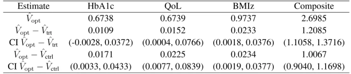
Table 2.1 depicts two measures of interest for evaluating the RLT ITR. The first measure is the estimated value ofV across the composite outcome and each univariate outcome. The second is the comparison between the value of the estimated optimal ITR and the fixed treatment effects for both intervention and usual care, which are computed asV withπ(X)assigning interven-tion or usual care to all patients, respectively. Note that each column of this table has a different natural scale due to the particular distribution of outcomes in question. All estimates of fixed treatment comparisons lie above zero, and all but one of the 95% confidence intervals lie entirely above zero, indicating the estimated optimal ITR achieved higher expected rewards than blanket assignment of treatment or usual care.
Estimate HbA1c QoL BMIz Composite
ˆ
Vopt 0.6738 0.6739 0.9737 2.6985
ˆ
Vopt−Vˆtrt 0.0109 0.0152 0.0233 1.2085
CIVˆopt−Vˆtrt (-0.0028, 0.0372) (0.0004, 0.0766) (0.0018, 0.0376) (1.1058, 1.3716) ˆ
Vopt−Vˆctrl 0.0171 0.0225 0.0234 1.0067
Table 3A-D also depicts the characteristics found to be significantly different across FLEX participants in the subgroups assigned to Intervention and Usual Care for the composite outcome and each univariate outcome. For full descriptive tables, please see Table S8. With the exception of the composite outcome, a large number of participants were assigned to the Muted Group.
Regarding the composite outcome, 91 participants (42%) were assigned to the Intervention, while the remaining 125 participants (58%) were assigned to the Control Group. Individuals assigned to intervention subgroup were less likely to have private health insurance (60% in the Intervention Group versus 78% in the Control Group,P = 0.01) (Table 3A).
Regarding the HbA1c univariate outcome, 105 participants (49%) were assigned to the Muted Group, 54 participants (25%) were assigned to the Intervention Group, and 57 partici-pants (26%) were assigned to the Control Group. Individuals assigned to the Intervention Group did not have a significantly higher Hba1c than those assigned to Usual Care (9.4% versus 9.2%; P = 0.44), but individuals in the Muted Group had higher mean HbA1c at baseline than those assigned to Intervention or Control (9.9%;P = 0.02andP < 0.01, respectively). Individuals in the Muted group also had a higher incidence of clinical and clinically serious hypoglycemia (P < 0.01), with no significant differences between the Intervention and Control Group (Table 3B).
Regarding the QoL univariate outcome, 63 participants (29%) were assigned to the Muted Group, 89 participants (41%) were assigned to the Intervention Group, and 64 participants (30%) were assigned to the Control Group. Individuals in the Intervention Group were more likely to have an elevated HbA1c at baseline compared to the Muted Group (75% versus 54%,P = 0.01) but not the Control Group (61%;P = 0.08). Individuals in the Intervention Group also had higher significantly higher depressive symptoms at baseline compared to those in the Muted Group (mean (SD) CESD 9.8 (8.5) versus mean (SD) CESD score 6.9 (5.4);P <0.01), with no significant differences from the Control Group (P = 0.44) (Table 3C).
were assigned to the Control Group. Mean BMIz at baseline of individuals assigned to the In-tervention Group was higher than that of those assigned to the Control Group (P < 0.01); this group also had a higher proportion of under- or normal weight individuals using weight status cut-offs (54.6% versus 30.6%;P < 0.01). Mean BMIz was not significantly different between the Intervention Group and the Control Group (P = 0.06; Table 3D).
2.4 Discussion
In this study, we present a method to identify subgroups of participants in a clinical trial for whom the studied intervention would have been beneficial, for whom the usual care condition would have been beneficial, and for whom the intervention did not make a difference, with re-gards to key clinical outcomes. We then apply this method to re-analyze data from the FLEX trial, which showed no effects of the intervention on the primary study outcome, to demonstrate that there are distinct subgroups with different optimal treatment assignments. We focus the dis-cussion first on the findings from thepost hocanalysis of the FLEX trial, and then turn to a more general discussion of the method itself.
The application of a method to find distinct subgroups within a single randomized trial sam-ple is appropriate given previous reports of heterogeneity in response to behavioral interventions (Hampson et al., 2000), including heterogeneity of response to the same intervention in different samples of youths with T1D (Channon et al., 2007; Wang et al., 2010). The relative proportions of these subgroups, especially with regards to the large muted group for HbA1c as a univariate outcome, highlight the challenges with glycemic control in this age range (Mayer-Davis et al., 2018b). By contrast, a larger group was estimated to benefit from the FLEX intervention with regards to QoL, which agrees with the main trial’s findings that the FLEX intervention had a positive aggregate effect on multiple measures of psychosocial well-being (Mayer-Davis et al., 2018b).
ben-efit take a central role in precision application of interventions (Kichler et al., 2018); as such, it would be ideal to have a large variety of markers corresponding to differential estimated response patterns (Trusheim et al., 2007; Khoury et al., 2012). Although we considered a range of par-ticipant characteristics, in the FLEX study, only a limited subset of characteristics emerged to distinguish the ITR-assigned subgroups. Furthermore, the markers were not consistent across the three univariate outcomes. For example, patients expected to be indifferent to intervention when optimizing for 18-month improvement in HbA1c had higher baseline HbA1c, while patients ex-pected to benefit more from intervention when optimizing for 18-month improvement in QoL had higher HbA1c at baseline. We believe these antagonistic effects may contribute to the paucity of reliable predictors for the subgroups governed by the composite outcome, even among covariates that helped predict subgroups for subgroups governed by univariate outcomes.
into this category, as these represent the population who may be the most difficult to reach via intervention work and may be at the highest risk of long-term complications of the disease.
This analysis is conceptually and analytically distinct from standard subgroup analysis meth-ods, representing a novel approach to subgroup determination. There are several advantages to this method forpost hocanalysis of randomized trial data. First, in contrast to descriptive meth-ods such as effect modification analysis, which show how treatment response differs across levels of a third modifying variable, this method is prescriptive, determining patients for whom the intervention is expected to be most beneficial. Second, unlike common approaches that start witha prioridefined subgroups and identify optimal treatment rules for each group, this analysis identifies an optimal treatment strategy across the entire study sample and uses it to determine subgroups of interest. As these subgroups are not specifieda prioribased on hypothesized mech-anism of disease, they may represent previously uncharacterized subgroups that are nevertheless relevant to the optimal delivery of intervention. Moreover, the data-driven nature of this method may help remove “researcher degrees of freedom” that can hinder reproducibility (Ioannidis, 2005; Simmons et al., 2011). Third, estimating an optimal ITR pools information from the entire study sample, not just the arm randomized to intervention. Finally, RLT allows us to model the intervention effect with a remarkably small number of assumptions, and its ability to handle high dimensionality allows us to consider a broad range of participant characteristics as suitable clini-cal markers, including aspects of cliniclini-cal care, sociodemographic characteristics, and behavioral measures at baseline that may reinforce or challenge the efficacy of a given therapy over time (Khoury et al., 2012).
promote adherence and improve glycemic control among youth with T1D. The precision delivery of interventions, based on a diverse breadth of data, as modeled in this study, offers a promising road forward.
2.5 Measures
In this section, we present details surrounding the measurement of key variables in the FLEX trial. We first give the details of measurement methodology for several covariates and outcomes. We then present the mathematical definitions of the four outcome variables used for our ITR estimation methods.
2.5.1 Measurement Methodology
Standardized Measurements
All data collection was standardized as per FLEX study protocol, and FLEX assessment staff were trained and certified to perform all study procedures. Adolescents and participating care-givers could choose to complete questionnaires online, through the secure FLEX study website, or during in-person study measurement visits. The full set of study measurements was obtained at baseline and 6 and 18 months post-randomization; a limited set of measurements was obtained at 3 and 9 months post-randomization (Mayer-Davis et al., 2018b).
Laboratory data
eight hours. LDL cholesterol was calculated by the Friedewald equation for those with triglyc-erides<4.52 mmol/l and by the beta-quantification procedure for those with triglycerides>4.52 mmol/l.
Clinical measures
At baseline and at 6- and 18-months post-randomization, patients wore a blinded CGM (iPro®2 Professional CGM; Medtronic Diabetes, Northridge, CA) for a seven-day period to mea-sure interstitial glucose levels in real time throughout the day and night. Cut-points for glucose used to describe hypoglycemia were established according to recommended values (Danne et al., 2017). Height was measured using a stadiometer, and weight was measured to the nearest 0.1 kg using an electronic scale. Body mass index (BMI, weight (kg) / height2(m2)) was calculated and converted to an age- and sex-specific BMI z-score (BMIz) according to Centers for Disease Control and Prevention growth charts. Blood pressure was measured after five minutes of rest using an aneroid manometer. The second and third of three measures were averaged for systolic and diastolic pressures.
Questionnaires
Patients self-reported race, highest level of parental education, duration of diabetes, insulin delivery method (pump versus multiple daily injections (MDI)), and past use of CGM outside the study in standardized questionnaires. Self-reported race and ethnicity was classified as non-Hispanic white, non-non-Hispanic Black, Black, and other including Asian/Pacific Islander, Native American, or unknown.
to be administered regardless of insulin regimen. Symptoms of depression were assessed using the Centers for Epidemiologic Study Depression Scale (CES-D), with higher scores reflecting more depressive symptoms (Radloff, 1977). The composite Pediatric Quality of Life InventoryTM Generic Core Scales (PedsQLTM) was used to assess quality of life (QoL) across four domains (physical, emotional, social, and school functioning) during the previous month, with higher scores reflecting better QoL (Varni et al., 2001). Fear of hypoglycemia was completed by both the adolescent and parents and measured three domains (Shepard et al., 2014): maintaining high blood sugar, helplessness/worry about low blood sugar, and worry about negative social conse-quences.
2.5.2 Outcome Variables
We first introduce notation that will be helpful in our mathematical definitions. LetR1,0 and
R1,1 denote the vector of patient HbA1c at baseline and 18 months, respectively. LetR2,0and
R2,1 denote the vector of patient quality of life, as determined by the PedsQL Generic scale, at
baseline and 18 months, respectively. Finally, letR3,0 andR3,1 denote the vector of patient BMI
Z-score at baseline and 18 months respectively. Leti = 1, . . . , nindex patients, such thatR1,0,i denotes patienti’s HbA1c at baseline, and so on.
We will define the three univariate outcomes before presenting the definition of the compos-ite outcome.
2.5.2.1 HbA1c univariate outcome
The raw univariate outcome vector for HbA1c is simply given byR1,raw = R1,1 −R1,0, i.e.
By convention, the clinical reward in ITR estimation settings is strictly positive, with larger values corresponding to better rewards. As such, we define the scaled univariate HbA1c outcome as follows:
R1 =
max(R1,raw)−R1,raw max(R1,raw)−min(R1,raw)
. (2.2)
Note that by definitionR1is restricted between 1 and 0, with larger values corresponding to
better outcomes (i.e. greater reductions in HbA1c).
2.5.2.2 QoL univariate outcome
The raw univariate outcome vector for quality of life is given byR2,raw=R2,1−R2,0, i.e. the
diffence between QoL scores at baseline and at 18 months. The raw univariate outcome is scaled such that more positive values are preferable, as they correspond to the largest increases in QoL.
By convention, the clinical reward in ITR estimation settings is strictly positive, with larger values corresponding to better rewards. As such, we define the scaled univariate QoL outcome as follows:
R2 =
R2,raw−min(R2,raw) max(R2,raw)−min(R2,raw)
. (2.3)
Note that by definitionR2is restricted between 1 and 0, with larger values corresponding to
better outcomes (i.e. larger increases in QoL).
2.5.2.3 BMIz univariate outcome
While the raw univariate outcome for BMIz,R3,raw = R3,1 −R3,0, offers computational
period. Giving these patients a poor clinical reward is inappropriate given the relationship be-tween glycemic control and body weight and the goals of the study. As such, we define the BMIz outcome to selectively penalize weight gain that results in excess body weight in relation to sex-and age-specific BMI percentiles. LetR36=1be the subvector ofR3,rawcorresponding to allisuch thatR3,1,i ≥ 1.04andR3,1,i > R3,0,ifor eachi. As such, we consider the following constrained BMIz outcome:
R3 =
1, ifR3,1 <1.04
1, ifR3,1−R3,0 <0
max(R6=13 )−R3,raw
max(R6=13 )−min(R6=13 ), otherwise.
(2.4)
By definition,R3 is constrained to lie between 0 and 1, with larger values corresponding to better
outcomes.
2.5.2.4 Composite Outcome
fail-ure criteria can be circumvented by strong enough improvement—for instance, a patient whose HbA1c at 18 months is 9.0 but whose HbA1c fell by 0.7 over the course of the intervention is not considered to have failed HbA1c for the purposes of the composite outcome.
We define the mutually exclusive outcome threshold eventsE1, E2, E3to simplify notation.
E1 is the indicator thatR1,1 > 8.5andR1,1 −R1,0 > 0.5.E2 is the indicator thatE1 = 0,
R2,1 <60, andR2,1−R2,0 <10.E3 is the indicator that bothE1 andE2equal 0. The thresholds
for HbA1c were chosen based on clinical cut-points, and the thresholds for QoL were chosen based on sample quantiles of QoL in the sample. The composite outcome is defined as follows:
R =
R1,1−8.5
max(R1,1)−8.5
, E1 = 1
1 + 60−R2,1 60−min(R2,1)
, E2 = 1
2 +R3, E3 = 1.
(2.5)
2.6 Properties of composite outcome
As the mathematical definition presented in 2.5.2.4 suggests, the distribution of the com-posite outcome depends directly upon an explicit hierarchy of the outcome variables in a trial, as well as meaningful regional thresholds that define failure events for those outcome variables. Both the hierarchy and the thresholds rely on domain knowledge. In the FLEX trial, for instance, domain knowledge suggested the regions of interest for one of our outcome variables—HbA1c below 8.5 is considered a significant improvement for this population, which was recruited with high baseline HbA1c (Association, 2016)—and informed the other, while the priorities of the trial dictated the order of the hierarchy. HbA1c was prioritized highest, as it was the outcome of primary interest and directly related to long-term complications of diabetes. QoL was prioritized second, as it was an outcome of secondary interest and represents an important patient-oriented outcome. Due to natural growth in this age range complicating BMI-based outcomes, and due to the complicated relationship between body weight and glycemic control alluded to in Sec-tion 2.5.2.3, BMIz was prioritized after both HbA1c and QoL (Mayer-Davis et al., 2018b). Note that the shape of the regions need not always be as simple as those presented in the FLEX trial— failure thresholds for raw BMI, for example, would likely penalize measurements that are too high as well as those that are too low.
2.6.1 Numerical Experiments
We examine the finite-sample performance of the composite outcome for ITR-based sub-group determination in a trial with heterogeneous treatment effects through a brief set of numer-ical experiments. In the first, we examine a very simple model to explore the properties of the method and the composite outcome, particularly regarding the muted group. In the second, we examine the performance of the method in settings more akin to those likely to be observed in real studies, paying special attention to comparing the performance of RLT and OWL-based subgroups.
Several features are similar across experiments. In both cases, the covariatesXare drawn i.i.d. fromU(−1,1), with a corresponding Gaussianp+ 1-vectorβthat governs the baseline link between covariates and clinical rewardR. The observed treatmentAis chosen independent of covariates and rewards so that patients are randomized equally to intervention (Ai = 1) and control (Ai = −1). Each experiment has two clinical rewards,R1 andR2. We specify true
sub-groups for each patient, stored in then-vectorS, whereSi ∈ {−1,0,1}denotes whether the patient benefits from control, has identical reward under control and treatment, or benefits from treatment, respectively. We assume that these subgroups apply to each outcome for the sake of simplifying comparisons to the gold standard; the details of how each subgroup is determined varies between experiments.R1 andR2 are constructed similarly across experiments. Given fixed
treatment effectsδ1andδ2forR1 andR2respectively, each experiment considers two settings. In
the first, termedsynergistic, the treatment effects point in the same direction for both outcomes:
forj = 1,2. In the reverse scenario, termedantagonistic, the treatment effects point in opposite ways for the two outcomes:
R1 =Xβ++δ1AS (2.7)
R2 =Xβ+−δ2AS.
The thresholdqdefines the failure event forR1: patients withR1 < qhave “failed”R1and
receive composite outcomeR ∈ [0,1]based on the magnitude of theirR1, while patients with
R1 ≥ qhave “acceptable”R1and receiveR ∈ [1,2]based on the magnitude of theirR2, in the
manner described in Section 2.5.2.4. We setqto the first quartile ofR1in the sequel. In each
simulation, once the data were generated, we estimated the optimal ITR in the sample using RLT (and, in the second experiment, OWL), then used it to obtain subgroup estimatesS. One set ofˆ evaluation metrics for the method is the subgroup recovery sensitivity and specificity, defined as
sensj =
Pn
i=1( ˆSi =j ∩Si =j)
Pn
i=1Si =j
(2.8)
specj =
Pn
i=1( ˆSi 6=j ∩Si 6=j)
Pn
i=1Si 6=j
,
wherej =−1,0,1. Another evaluation metric is available for the RLT ITR due to the simulated nature of the data. LetR1andR−1denote the true value ofRunder intervention and control. Since we know the magnitude and direction of the true treatment effect for bothR1 andR2, we
can calculate the difference inRobtained by switching a patient on intervention to control or vice versa. For instance, in the synergistic setting, a patient withSi = 1andAi = 1would have Ri−11 =Ri1−δ1 andRi−21 =Ri2−δ2. ThenR−i 1 could be obtained by recalculatingRin the manner described in (2.5) with these perturbed values. LetQˆ1(X)andQˆ−1(X)denote the RLT-predicted
error in treatment effect, defined as
MSE=n−1 n
X
i=1 h
R1i −Ri−1−Qˆ1(Xi)−Qˆ−1(Xi)
i2
. (2.9)
2.6.1.1 Experiment in Simple Conditions
We first explored a basic model to assess the performance of the method when when all factors are straightforward, particularly with regards to the muted group. In this model, we set n= 200andp= 1.
As briefly discussed in Section 2.6.1, we intentionally built a muted group into our simulated data. In particular, we allotted the true subgroup membership according to
S =
1, X >0.5
−1, X <−0.5 0, otherwise.
(2.10)
In this experiment, we considered both the synergistic and antagonistic setting, and we consid-ered three values for eachδj: 1, 3, and 10.
As our goal in this simulation was to examine the behavior of the method surrounding the muted group, we used only RLT to estimate the optimal ITR.
Table 2.2 gives the subgroup recovery sensitivity and specificity in the synergistic setting byδ1,δ2, and value ofS. Overall, we see high sensitivity for both the intervention and control
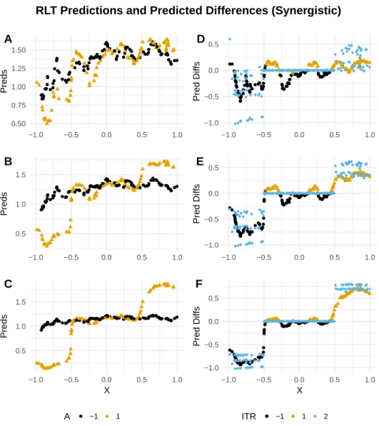
large, which suggests the method is performing well. Figure 2.1 illustrates the disconnect be-tween the conclusions drawn from these evaluation metrics. In particular, whenXi ∈[−0.5,0.5], we knowSi = 0, so a method that performs perfectly would haveQˆ1(Xi)−Qˆ−1(Xi)within this range. The method does not set any of these differences identically equal to zero for any combina-tion of(δ1, δ2); however, for each(δ1, δ2), the estimated differences are smaller in this range than
outside it, with this trend increasing as the true treatment effect increases. We will return to this observation in our discussion in Section 2.6.1.3.
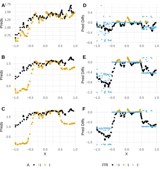
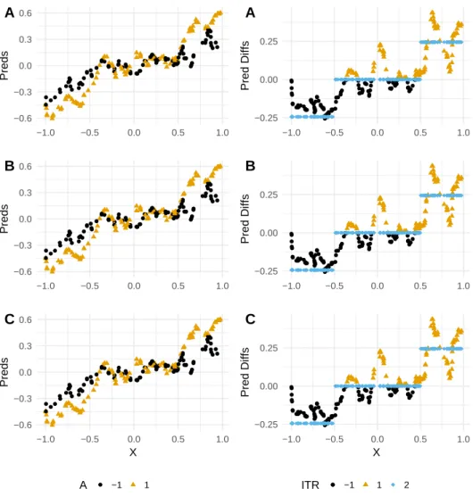
Table 2.4 gives the treatment effect MSE in the antagonistic setting. Again, MSE is low throughout, suggesting the method performs well even in this conceptually more difficult setting. Figure 2.2 illustrates the predictions and estimated vs. true treatment effects plotted against the true splitting variableX in the antagonistic setting. Again, the predicted differences between interention and control are smaller in magnitude inside the range of the true muted group than outside it, on average, though none are set identically to zero. We also note the somewhat unintu-itive behavior of the true treatment effects: although the treatment effect is truly posunintu-itive for one of the outcome variables, nearly all the true treatment effects are negative. Optimizing on either outcome in a univariate manner would fail to discover this interesting trend, as Figure 2.3 demon-strates: the trend for the univariate outcome appears similar to that exhibited in the synergistic setting.
2.6.1.2 Experiment in Trial-Like Conditions
RLT Predictions and Predicted Differences (Synergistic) ● ● ● ● ● ● ● ● ● ● ● ● ● ● ● ● ● ● ● ● ● ● ● ● ● ● ● ● ● ● ● ● ● ● ● ● ● ● ● ● ●● ● ● ● ● ● ● ● ● ● ● ● ● ● ● ● ● ● ● ● ● ● ● ● ● ● ● ● ● ● ● ● ● ● ● ● ● ● ● ● ● ● ● ● ● ● ● ● ● ● ● ● ● ● ● ● ● ● ● 0.50 0.75 1.00 1.25 1.50
−1.0 −0.5 0.0 0.5 1.0
Preds A ● ● ● ● ● ● ● ● ● ● ● ● ● ● ● ● ● ● ● ● ● ● ● ● ● ● ● ● ● ● ● ● ● ● ● ● ● ● ● ● ●● ● ● ● ● ● ● ● ● ● ● ● ● ● ● ● ● ● ● ● ● ● ● ● ● ● ● ● ● ● ● ● ● ● ● ● ● ● ● ● ● ● ● ● ● ● ● ● ● ● ● ● ● ● ● ● ● ● ● 0.5 1.0 1.5
−1.0 −0.5 0.0 0.5 1.0
Preds B ● ● ● ● ● ● ● ● ● ● ● ● ● ● ●● ● ● ● ● ● ● ● ● ● ● ● ● ● ● ● ● ● ● ● ● ● ● ●●●● ● ● ● ● ●● ● ● ● ● ● ● ● ● ● ● ● ● ● ● ● ● ● ●● ● ● ● ● ● ● ● ● ● ● ● ● ● ● ● ● ● ● ● ● ● ● ● ● ● ● ● ● ● ● ● ● ● 0.5 1.0 1.5
−1.0 −0.5 0.0 0.5 1.0
X
Preds
C
A ● −1 1
● ● ● ● ● ● ● ● ● ● ● ● ● ● ●● ● ● ● ● ● ● ● ●●● ● ● ● ● ● ● ● ● ● ●● ● ● ● ● ● ● ● ● ● ● ● ● ● ● ● ● ● ● ● ● ● ● ● ● ● ● ● ● ● ● ● ● ● ● ● ● ● ● ● ● ● ● ● ● ● ● ● ● ● ● ● ● ● ● ● ● ● ● ● ●● ● ● ● ● ● ● ● ● ● ● ● ● ● ● ● −1.0 −0.5 0.0 0.5
−1.0 −0.5 0.0 0.5 1.0
Pred Diffs D ● ● ● ● ● ● ● ● ● ● ● ● ● ● ●● ● ● ● ● ● ● ●● ●●● ● ● ● ● ● ● ● ● ●● ● ● ● ● ● ● ● ● ● ● ● ● ● ● ● ● ● ● ● ● ● ● ● ● ● ● ● ● ● ● ● ● ● ● ● ● ● ● ● ● ● ● ● ● ● ● ● ● ● ● ● ● ● ● ● ● ● ● ● ●● ● ● ● ● ● ● ● ● ● ● ● ● ● ● ● −1.0 −0.5 0.0 0.5
−1.0 −0.5 0.0 0.5 1.0
Pred Diffs E ● ● ● ● ● ● ● ● ● ● ● ● ● ● ●● ● ● ● ● ● ● ●● ●●● ● ● ● ● ● ● ● ● ● ● ● ● ● ● ● ● ● ● ● ● ● ● ● ●● ● ● ● ● ● ●●● ● ● ● ● ● ● ● ● ● ●● ● ● ● ● ● ● ● ● ● ● ● ● ● ● ● ● ● ● ● ● ● ● ● ● ● ●● ● ● ● ● ● ● ● ● ● ● ● ● ● ● ● −1.0 −0.5 0.0 0.5
−1.0 −0.5 0.0 0.5 1.0
X
Pred Diffs
F
ITR ●● −1 1 2
Figure 2.1: (A-C). RLT-predicted values ofRby true treatment effect, intervention status, and true splitting variableXfor the simple numerical experiment of Section 2.6.1.1, synergistic setting. The true treatment effects forR1andR2are set toδ1 = δ2 = 1,3,10in A, B, and C, respectively. (D-F). Differences in predicted composite rewardRbetween intervention and control by true treatment effect, RLT ITR assignment, and true splitting variable
RLT Predictions and Predicted Differences (Antagonistic) ● ● ● ● ● ● ● ● ● ● ● ● ● ● ● ● ● ● ● ●● ● ● ● ● ● ● ● ● ● ● ● ● ● ● ● ● ● ● ● ● ● ● ● ● ● ● ● ● ● ● ● ● ● ● ● ● ● ● ● ● ● ● ● ● ● ● ● ● ● ● ● ● ● ● ● ● ● ● ● ● ● ● ● ● ● ● ● ● ● ●● ● ● ● ● ● ● ● ● 0.75 1.00 1.25 1.50 1.75
−1.0 −0.5 0.0 0.5 1.0
Preds A ● ● ● ● ● ● ● ● ● ● ● ● ● ● ● ● ● ● ● ● ● ● ● ● ● ● ● ● ● ● ● ● ● ● ● ● ● ● ● ● ●● ● ● ● ● ● ● ● ● ● ● ● ● ● ● ● ● ● ● ● ● ● ● ● ● ● ● ● ● ● ● ● ● ● ● ● ● ● ● ● ● ● ● ● ● ● ● ● ● ●● ● ● ● ● ● ● ● ● 0.5 1.0 1.5
−1.0 −0.5 0.0 0.5 1.0
Preds B ●● ● ● ● ● ● ● ● ● ● ● ● ● ● ● ● ● ● ●● ● ● ● ● ● ● ● ● ● ● ● ● ● ● ● ● ● ● ● ●● ● ● ● ● ● ● ● ● ● ● ● ● ● ● ● ● ● ● ● ● ● ● ● ● ● ● ● ● ● ● ● ● ● ● ● ● ● ● ● ● ● ● ● ● ● ● ● ● ●● ● ● ● ● ● ● ● ● 0.5 1.0 1.5
−1.0 −0.5 0.0 0.5 1.0
X
Preds
C
A ● −1 1
● ● ● ● ● ● ● ● ● ● ● ● ● ● ● ● ● ● ● ● ● ● ● ● ● ● ● ● ● ● ● ● ● ● ● ● ● ● ● ● ● ● ● ● ● ● ● ● ● ● ● ● ● ● ● ● ● ● ● ● ● ● ● ● ● ● ● ● ● ● ● ● ● ● ● ● ●● ●● ● ● ● ●● ● ● ● ● ● ● ● ● ● ● ●● ● ● ● ● ● ● ● ● ● ● ● ● ● ● ● ● ● ● ● ● ● ● ● ● ● ● ● ● ● ● ● ● ● ● ● ● ● ● ●● ● ● ● ● ● ● ● ● ●● ● ● ● ● ● ● ● ● ● ● ● ● −0.8 −0.4 0.0 0.4
−1.0 −0.5 0.0 0.5 1.0
Pred Diffs D ● ● ● ● ● ● ● ● ● ● ● ● ● ● ● ● ● ● ● ● ● ● ● ● ● ● ● ● ● ● ● ● ● ● ● ● ● ● ● ● ● ● ● ● ● ● ● ● ● ● ● ● ● ● ● ● ● ● ● ● ● ● ● ● ● ● ● ● ● ● ● ● ● ● ● ● ● ● ● ● ● ● ● ●● ● ● ●● ● ● ● ● ● ● ● ● ● ● ● ●● ● ● ● ● ● ●● ● ● ● ● ● ● ● ● ● ● ● ● ● ● ● ● ● ● ● ● ● ● ● ● ● ● ● ● ● ● ● ● ● ● ● ● ● ● ● ● ● ● ● ● ● ● ● ● ● ● ● ● ● ● ● ● ● ● −1.2 −0.8 −0.4 0.0
−1.0 −0.5 0.0 0.5 1.0
Pred Diffs E ●● ● ● ● ● ● ● ● ● ● ● ● ● ● ● ● ● ● ● ● ● ● ● ● ● ● ● ● ● ● ● ● ● ● ● ● ● ● ● ● ● ● ● ● ● ● ● ● ● ● ● ● ● ● ● ● ● ● ● ● ● ● ● ● ● ● ● ● ● ● ● ● ● ● ● ● ● ● ●● ● ● ●● ● ● ● ● ● ● ● ● ● ● ● ●● ● ●● ● ● ● ● ● ● ● ● ● ● ● ● ● ● ● ● ● ● ● ● ● ● ● ● ● ● ● ● ● ● ● ● ● ● ● ● ● ● ● ● ● ● ● ● ● ● ● ● ● ● ● ● ● ● ● ● ● ● ● ● ● ● ● ● −1.5 −1.0 −0.5 0.0
−1.0 −0.5 0.0 0.5 1.0
X
Pred Diffs
F
ITR ●● −1 1 2
Figure 2.2: (A-C). RLT-predicted values ofRby true treatment effect, intervention status, and true splitting variableXfor the simple numerical experiment of Section 2.6.1.1, antagonistic setting. The true treatment effects forR1andR2are set toδ1 = δ2 = 1,3,10in A, B, and C, respectively. (D-F). Differences in predicted composite rewardRbetween intervention and control by true treatment effect, RLT ITR assignment, and true splitting variable
Univariate Predictions and Predicted Differences (Antagonistic) ● ● ● ● ● ● ● ● ● ● ● ● ● ● ● ● ● ● ● ● ● ● ● ● ● ● ● ● ● ● ● ● ● ● ● ● ● ● ● ● ● ● ● ● ● ● ● ● ● ● ● ● ● ● ● ● ● ● ● ● ● ● ● ● ● ● ● ● ● ● ● ● ● ● ● ● ● ● ● ● ● ● ● ● ● ● ● ● ● ● ●● ● ● ● ● ● ● ● ● −0.6 −0.3 0.0 0.3 0.6
−1.0 −0.5 0.0 0.5 1.0
Preds A ● ● ● ● ● ● ● ● ● ● ● ● ● ● ● ● ● ● ● ● ● ● ● ● ● ● ● ● ● ● ● ● ● ● ● ● ● ● ● ● ● ● ● ● ● ● ● ● ● ● ● ● ● ● ● ● ● ● ● ● ● ● ● ● ● ● ● ● ● ● ● ● ● ● ● ● ● ● ● ● ● ● ● ● ● ● ● ● ● ● ●● ● ● ● ● ● ● ● ● −0.6 −0.3 0.0 0.3 0.6
−1.0 −0.5 0.0 0.5 1.0
Preds B ● ● ● ● ● ● ● ● ● ● ● ● ● ● ● ● ● ● ● ● ● ● ● ● ● ● ● ● ● ● ● ● ● ● ● ● ● ● ● ● ● ● ● ● ● ● ● ● ● ● ● ● ● ● ● ● ● ● ● ● ● ● ● ● ● ● ● ● ● ● ● ● ● ● ● ● ● ● ● ● ● ● ● ● ● ● ● ● ● ● ●● ● ● ● ● ● ● ● ● −0.6 −0.3 0.0 0.3 0.6
−1.0 −0.5 0.0 0.5 1.0
X
Preds
C
A ● −1 1
● ● ● ● ● ● ● ● ● ● ● ● ● ● ● ● ● ● ● ● ● ● ● ● ● ● ● ● ● ● ● ● ● ● ● ● ● ● ● ● ● ● ● ● ● ● ●●● ● ● ● ● ● ● ● ● ● ● ● ● ● ●● ● ● ● ● ● ● ● ● ● ● ● ● ● ● ● ● ● ● ●● ● ● ● ● ● ● ● ● ● ● ● ● ● −0.25 0.00 0.25
−1.0 −0.5 0.0 0.5 1.0
Pred Diffs A ● ● ● ● ● ● ● ● ● ● ● ● ● ● ● ● ● ● ● ● ● ● ● ● ● ● ● ● ● ● ● ● ● ● ● ● ● ● ● ● ● ● ● ● ● ● ●●● ● ● ● ● ● ● ● ● ● ● ● ● ● ●● ● ● ● ● ● ● ● ● ● ● ● ● ● ● ● ● ● ● ●● ● ● ● ● ● ● ● ● ● ● ● ● ● −0.25 0.00 0.25
−1.0 −0.5 0.0 0.5 1.0
Pred Diffs B ● ● ● ● ● ● ● ● ● ● ● ● ● ● ● ● ● ● ● ● ● ● ● ● ● ● ● ● ● ● ● ● ● ● ● ● ● ● ● ● ● ● ● ● ● ● ●●● ● ● ● ● ● ● ● ● ● ● ● ● ● ●● ● ● ● ● ● ● ● ● ● ● ● ● ● ● ● ● ● ● ●● ● ● ● ● ● ● ● ● ● ● ● ● ● −0.25 0.00 0.25
−1.0 −0.5 0.0 0.5 1.0
X
Pred Diffs
C
ITR ●● −1 1 2
δ1 δ2 Measure S =−1 S= 0 S = 1
1 1 Sens 0.962 0.000 0.917
Spec 0.541 1.000 0.750
3 Sens 0.981 0.000 1.000
Spec 0.581 1.000 0.743
10 Sens 1.000 0.000 1.000
Spec 0.669 1.000 0.664
3 1 Sens 1.000 0.000 0.917
Spec 0.547 1.000 0.757
3 Sens 1.000 0.000 1.000
Spec 0.581 1.000 0.750
10 Sens 1.000 0.000 1.000
Spec 0.581 1.000 0.750
10 1 Sens 1.000 0.000 0.938
Spec 0.534 1.000 0.776
3 Sens 1.000 0.000 1.000
Spec 0.601 1.000 0.730
10 Sens 1.000 0.000 1.000
Spec 0.588 1.000 0.743
Table 2.2: Subgroup Recovery Sensitivity and Specificity by Treatment Effect (Simple Experi-ment, Synergistic Setting)
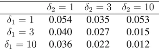
δ2 = 1 δ2 = 3 δ2 = 10
δ1 = 1 0.054 0.035 0.053
δ1 = 3 0.040 0.027 0.015
δ1 = 10 0.036 0.022 0.012
Table 2.3: Treatment Effect MSE by True Treatment Effect (Simple Experiment, Synergistic Setting)
As in the simple simulation of Section 2.6.1.1, we divide the sample into a true intervention, control, and muted group. The subgroup divisions are given by
S =
−1, atX
k,int< c1
1, atX
k,int> c2
0, otherwise,
(2.11)
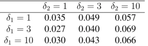
δ2 = 1 δ2 = 3 δ2 = 10
δ1 = 1 0.035 0.049 0.057
δ1 = 3 0.027 0.040 0.069
δ1 = 10 0.030 0.043 0.066
Table 2.4: Treatment Effect MSE by True Treatment Effect (Simple Experiment, Antagonistic Setting)
In the sequel, we choosek = 2and setc1 andc2 to the first and third quartiles ofaTXk,R,
respec-tively. In this experiment, we considered both the synergistic and antagonistic setting, and we considered three values for the true univariate treatment effectsδj, j = 1,2: 1, 3, and 10. Addi-tionally, we considered both RLT and OWL to estimate the optimal ITR. We ran 100 simulations for each combination of ITR method,δ1,δ2, and setting.
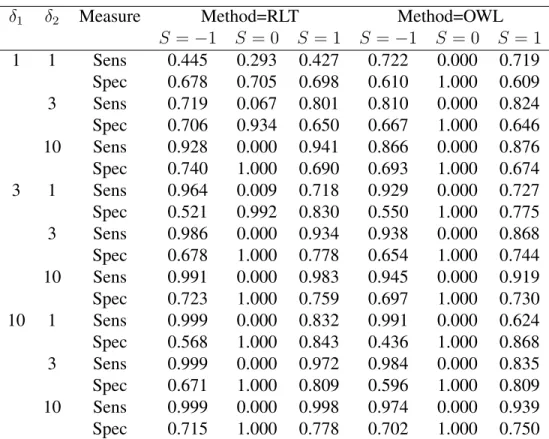
Table 2.5 gives the average subgroup recovery sensitivity and specificity over the 100 simula-tions for both RLT and OWL for the synergistic setting, divided by true subgroup status and true value of the univariate treatment effectsδ1 andδ2. Both methods show improvements in
sensitiv-ity for the intervention and control groups as the true treatment effect sizes increase. RLT once again struggles to pick up a muted group in any setting, failing to do so entirely when effect sizes are large. Unlike in the numerical experiment of Section 2.6.1.1, RLT does succeed in discover-ing a muted group with high specificity when effect sizes are small, albeit with modest sensitivity. As noted before, OWL is incapable of discovering a muted group; its sensitivity and specificity remain admirably high in the groups it can recover.
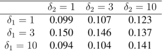
Tables 2.6 and 2.7 give the average treatment effect MSE over the 100 simulations by true value of univariate treatment effectsδ1andδ2 for the synergistic and antagonistic settings,
δ1 δ2 Measure Method=RLT Method=OWL
S =−1 S = 0 S = 1 S=−1 S = 0 S = 1
1 1 Sens 0.445 0.293 0.427 0.722 0.000 0.719
Spec 0.678 0.705 0.698 0.610 1.000 0.609
3 Sens 0.719 0.067 0.801 0.810 0.000 0.824
Spec 0.706 0.934 0.650 0.667 1.000 0.646
10 Sens 0.928 0.000 0.941 0.866 0.000 0.876
Spec 0.740 1.000 0.690 0.693 1.000 0.674
3 1 Sens 0.964 0.009 0.718 0.929 0.000 0.727
Spec 0.521 0.992 0.830 0.550 1.000 0.775
3 Sens 0.986 0.000 0.934 0.938 0.000 0.868
Spec 0.678 1.000 0.778 0.654 1.000 0.744
10 Sens 0.991 0.000 0.983 0.945 0.000 0.919
Spec 0.723 1.000 0.759 0.697 1.000 0.730
10 1 Sens 0.999 0.000 0.832 0.991 0.000 0.624
Spec 0.568 1.000 0.843 0.436 1.000 0.868
3 Sens 0.999 0.000 0.972 0.984 0.000 0.835
Spec 0.671 1.000 0.809 0.596 1.000 0.809
10 Sens 0.999 0.000 0.998 0.974 0.000 0.939
Spec 0.715 1.000 0.778 0.702 1.000 0.750
Table 2.5: Subgroup Recovery Sensitivity and Specificity by Method and Treatment Effect (Trial-Like Conditions, Synergistic Setting)
δ2 = 1 δ2 = 3 δ2 = 10
δ1 = 1 0.109 0.129 0.139
δ1 = 3 0.153 0.137 0.119
δ1 = 10 0.091 0.080 0.055
Table 2.6: Treatment Effect MSE by True Treatment Effect (Trial-Like Conditions, Synergistic Setting)
2.6.1.3 Discussion of Numerical Experiments
δ2 = 1 δ2 = 3 δ2 = 10
δ1 = 1 0.099 0.107 0.123
δ1 = 3 0.150 0.146 0.137
δ1 = 10 0.094 0.104 0.141
Table 2.7: Treatment Effect MSE by True Treatment Effect (Trial-Like Conditions, Antagonistic Setting)
much smaller treatment effects in the range defined by the muted group than the range defined by the intervention and control groups, but failed to set these effects identically equal to zero. An “-insensitive” version of the method, in which predicted values under treatment and control must differ by at leastto be placed into either the control or intervention group, might offer improved performance with the same attractive interpretability. As discussed more fully in Section 2.8, the implementation of OWL used here cannot create a muted group, but an-insensitive exten-sion of OWL might offer the same attractive features. For either potential-insensitive method, challenges prove to arise from determining the best automated procedure for choosing.
Another notable trend observed in the numerical experiments in both Sections 2.6.1.1 and 2.6.1.2 is the high specificity for the muted group even when effect sizes were small. This fact may increase our confidence in the existence of the muted group assigned by RLT in the FLEX trial, while the satisfactory sensitivity and specificity for both the intervention and control groups in numerical experiments is promising for those groups as well.
2.7 Sensitivity Analyses
Table 2.8 givesVˆoptfor each combination of dataset, ITR estimation method, and outcome
trained upon. Each column of table 2.8 has its own natural numerical scale, due to the distribu-tion of the underlying rewards. The combinadistribu-tion of method and dataset that performed the best for each outcome, in terms of value, is shown in bold. 95% confidence intervals for each value es-timate are given by the bootstrap, described in fuller detail in Section 2.9. For the three univariate outcomes, the different ITRs show only minor differences in value. OWL in the imputed dataset performs nominally best for HbA1c and QoL, while OWL in the complete cases performs nom-inally best for BMIz. Of these comparisons, only one seems to indicate a significant difference: RLT in the imputed dataset appears to perform worse than OWL in the imputed dataset for the univariate HbA1c outcome, with the former’s 95% CI lying entirely above the latter’s. For the composite outcome, however, RLT in the imputed dataset provides a substantial improvement in value over all other estimated ITRs, with its 95% CI lying well above all other ITR’s.
Dataset Method HbA1c QoL BMIz Composite
Complete cases RLT 0.6786 0.6434 0.9670 2.1359
(0.660,0.702) (0.643,0.702) (0.954,0.984) (2.030,2.272)
OWL 0.6905 0.7006 0.9857 2.0734
(0.693,0.707) (0.698,0.722) (0.984,0.989) (2.060,2.167)
Imputed RLT 0.6738 0.6739 0.9737 2.6985
(0.661,0.689) (0.669,0.722) (0.960,0.988) (2.696,2.858)
OWL 0.7044 0.7021 0.9855 1.9867
(0.702,0.705) (0.701,0.703) (0.985,0.986) (1.959,2.070) Table 2.8: Estimated Value (Bootstrap 95% Confidence Interval) of ITR by Method, Dataset, and Outcome Variable