SCISSOR FOR FINDING OUTLIERS IN RNA-SEQ
Hyo Young Choi
A dissertation submitted to the faculty of the University of North Carolina at Chapel Hill in partial fulfillment of the requirements for the degree of Doctor of Philosophy in the Department of
Statistics and Operations Research.
Chapel Hill 2018
ABSTRACT
Hyo Young Choi: Scissor for finding outliers in RNA-seq (Under the direction of J. S. Marron and D. Neil Hayes)
The impressive progress of high-throughput technologies has provided many interesting modern data types, which has tremendously increased the demand for Statistics. RNA-seq, in particular, allows a rich characterization of the genome with many exciting applications. This dissertation makes contributions to RNA-seq data analysis by addressing several statistical challenges especially characterized by high dimensionality.
The dissertation is composed of two major parts. The first part concerns the issue of high dimensional outliers which are challenging to distinguish from inliers due to the special structure of high dimensional space. We introduce a new notion of high dimensional outliers that embraces various types and provides deep insights into understanding the behavior of these outliers based on several asymptotic regimes. Using this new framework, we develop an outlier detection method called Scissor that aims to identify sample outliers with distinct forms or patterns of transcripts across RNA-seq cohorts. Scissor offers a novel approach to unsupervised screening of a variety of shape changes that are possibly associated with important genetic events. Scissor has been implemented inRand is available online.
TABLE OF CONTENTS
LIST OF TABLES . . . ix
LIST OF FIGURES . . . x
CHAPTER 1. INTRODUCTION . . . 1
1.1 High-dimensional asymptotics . . . 2
1.2 RNA-seq data . . . 6
1.3 Outline . . . 8
CHAPTER 2. THEORY OF HIGH-DIMENSIONAL OUTLIERS . . . 9
2.1 Motivation . . . 9
2.2 Related work . . . 11
2.3 Model and Notations . . . 13
2.4 Geometrical representation. . . 18
2.5 PCA consistency . . . 22
2.6 Illustration using a toy example . . . 31
2.7 Proofs . . . 34
2.7.1 Proof of Theorem 2.5.1 . . . 35
2.7.2 Proof of Theorem 2.5.2 . . . 42
CHAPTER 3. SCISSOR: SHAPE CHANGES IN SELECTING SAMPLE OUT-LIERS IN RNA-SEQ . . . 51
3.1 Motivation and Challenges . . . 51
3.2 Related work . . . 53
3.4 Pre-processing data . . . 57
3.4.1 Filtering out degraded samples . . . 61
3.4.2 Filtering out on/off genes . . . 63
3.4.3 Inclusion of intronic part . . . 70
3.4.4 Data transformation . . . 71
3.4.5 Data normalization . . . 74
3.5 Detecting shape changes . . . 78
3.5.1 Global shape change detection . . . 79
3.5.1.1 The most outlying direction . . . 79
3.5.1.2 Projection depth function with(µ,σ)=(Mean, SD) . . . 83
3.5.1.3 Projection depth function with(µ,σ)=(Med, MAD) . . . 86
3.5.1.4 Global shape change detection algorithm . . . 88
3.5.1.5 Analysis with toy example . . . 89
3.5.2 Local shape change detection . . . 91
3.6 Results. . . 94
3.6.1 Per-gene analysis . . . 94
3.6.1.1 TP53 . . . 94
3.6.1.2 CDKN2A . . . 103
3.6.2 Genome-wide analysis . . . 106
CHAPTER 4. DETERMINING THE NUMBER OF SPIKES IN PCA . . . 111
4.1 Motivation . . . 111
4.2 Related work . . . 112
4.3 Known results on the generalized spike covariance model . . . 114
4.4 Methodology . . . 117
4.4.1 Estimation when the PSD is known . . . 117
4.4.3 PSD diagnostics . . . 120
4.5 Real data analysis . . . 121
4.5.1 The proposed noise model . . . 123
4.5.2 Application to important genes . . . 125
LIST OF TABLES
2.1 Sample eigenvectors . . . 33
3.2 GO enrichment analysis of Cluster 2 . . . 69
3.3 Illustration of MODs using a high-dimensional toy example . . . 90
3.4 Mutational analysis at TP53 . . . 97
3.5 Mutational analysis at CDKN2A . . . 104
LIST OF FIGURES
1.1 Marcenko Pastur distribution . . . 3
2.2 TP53 RNA-seq data . . . 14
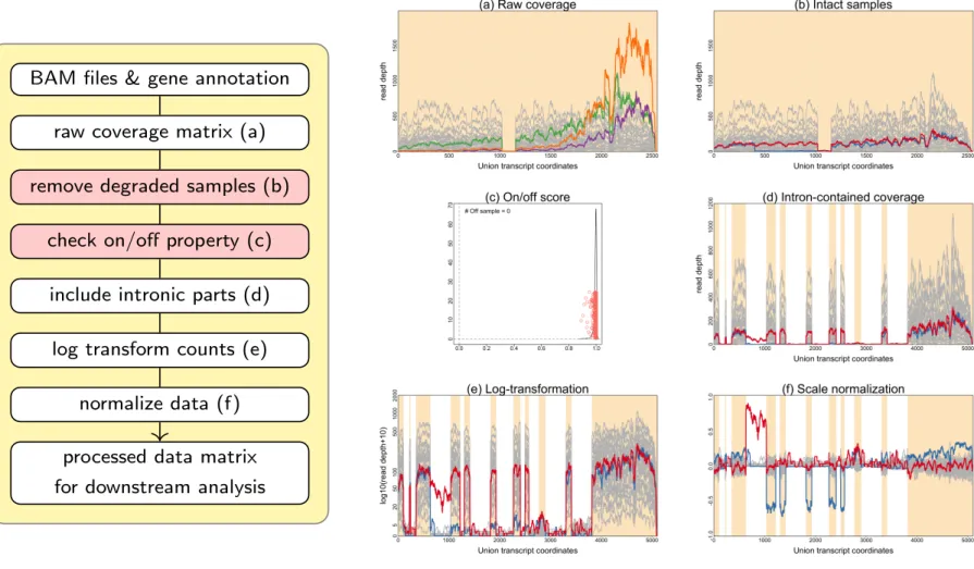
3.3 Pre-processing step . . . 60
3.4 Heatmap of decay rates . . . 62
3.5 Intact and degraded samples . . . 64
3.6 On/Off analysis at XIST . . . 66
3.7 On/Off gene analysis . . . 67
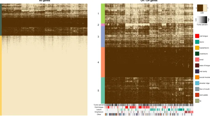
3.8 Heatmap of On/Off genes . . . 68
3.9 Data transformation . . . 73
3.10 Data normalization . . . 77
3.11 Illustration of MODs using a two-dimensional toy example . . . 81
3.12 Distribution of PO scores . . . 90
3.13 Outlier detection at TP53 . . . 95
3.14 Examples of global and local shape changes . . . 96
3.15 New variants identified from Scissor . . . 98
3.16 Identified shape changes associated with splice site mutations . . . 100
3.17 Identified shape changes associated with frameshift mutations . . . 101
3.18 Identified shape changes in the absent of mutations called . . . 102
3.19 Outlier detection at CDKN2A . . . 103
3.20 Identified splice mutations in CDKN2A . . . 104
3.21 Identified shape changes in the absence of splice site mutations . . . 105
3.22 Mutational analysis with the genome-wide results from Scissor . . . 106
3.23 Percentage of identified mutations in tumor suppressor genes and oncogenes . . . 107
3.24 Distribution of maximum scores . . . 108
4.26 Illustration of a psi function . . . 116
4.27 Examples of a psi envelope for assessment of the point mass PSDH=δ1. . . 121
4.28 RNA-seq data of CDKN2A . . . 122
4.29 Psi envelopes assuming white noise . . . 123
CHAPTER 1. INTRODUCTION
Through advancements in terms of computing speed, storage capability, and data-collection technologies, the scope of Data Science has profoundly broadened. An immeasurable amount of data have been generated at an unprecedented speed and a variety of new data types have emerged from numerous platforms such as social media sites, Internet of Things (IoT), and scientific research institutions. The emergence of such massive data, or Big Data, and new data structures has tremendously increased the demand of Statistics.
An important type of Big Data is often characterized by a large number of variables in the thousands, millions and more with only tens or hundreds of observations (large d, smalln). In statistical terminologies, we often call such a data set “high dimensional” or “large dimensional”. Among many statistical challenges raised by Big Data, high dimensionality is a major issue. In traditional data analysis, it is assumed that data consist of many observations and a relatively few variables (largen, smalld). The asymptotic assumption of increasingnwith a fixeddleads to nice theoretical properties such as consistency, efficiency, and asymptotic normality. However, such theories do not provide useful insights for large d data sets. For example, a sample covariance matrix is not a consistent estimator for the true one in the case of an increasingd even whennis large. This is mainly because the number of parameters to be estimated (d(d2+1)) is much larger than the number of observations (nd) (See Section 1.1).
dimensionality, tremendous efforts have been made in both theoretical and methodological statistics for the last few decades.
This dissertation makes further contributions to the high dimensional data analysis motivated by challenges arising from modern genomic data types. We explore several theoretical aspects of high dimensional data in some particular situations where regular assumptions are violated and develop new statistical tools based on the theories investigated.
1.1 High-dimensional asymptotics
The sample covariance matrix is one of the fundamental objects in multivariate data analysis. When the sample size tends to infinity and the dimension size is fixed, the sample covariance matrix can be used as a good estimate of the population covariance matrix. However, when the dimension size is large, the estimation of the population covariance matrix based on the sample covariance matrix can become very poor. To appreciate this issue, letX be ad×n data matrix whose columns are random vectors fromNd(0,Id)and denote a version of its sample covariance matrix bySn=1nXXT. Note that we do not subtract the sample mean vector because the population
mean is zero. In the classical domain when ntends to infinity andd is fixed, it is expected that the eigenvalues of Sn will be close to 1, which is the eigenvalue of the population covariance
matrix,Id, which is a sense thatSnis a good estimate ofId. Under different conditions, however, the
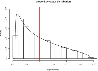
empirical distribution of the eigenvalues ofSnconverges to the Marcenko-Pastur (M-P) distribution
(Marˇcenko and Pastur, 1967), when d and nboth tend to infinity such that dn →c, as illustrated in Figure 1.1. The histogram illustrates the distribution of sample eigenvalues ofSnwithd=500
andn=1000. The curve indicates the theoretical M-P distribution withc=0.5. The distribution strongly deviates from the distribution of the population eigenvalue, which is a point mass at 1. This supports the idea that the sample covariance matrix is not a good estimate of the population covariance matrix for large dimensions.
Marcenko−Pastur distribution
Eigenvalues
Density
0.0 0.5 1.0 1.5 2.0 2.5 3.0
0.0
0.2
0.4
0.6
0.8
1.0
Figure 1.1: The histogram shows the empirical distribution of eigenvalues ofSnwithd=500 and
n=1000. The red vertical line indicates the distribution of the population eigenvalue, which is a point mass at 1. The curve shows the theoretical M-P distribution with an indexc=0.5. The empirical distribution well follows the theoretical M-P distribution whereas both distributions are strongly deviated from the population eigenvalue distribution.
sample eigenvalues is known to be a semi-circular law with an extreme point mass at zero. If dn →0 asdandnboth increase, the sample eigenvalues converge to one while the limiting distribution with suitable rescaling results in a semi-circular law. Thus, different asymptotic domains yield different limiting properties. Among various asymptotic regimes, this dissertation spotlights three asymptotic regimes:
• Classicalasymptotic regime considers an increasingn(n→∞) and fixedd.
• Random matrix theory (RMT)asymptotic regime considers proportionally increasing n andd, i.e.n→∞andd→∞such that dn →c. Here,cis mostly assumed to be a constant within 0<c<∞.
• High dimensional low sample size (HDLSS)asymptotic regime considers an increasingd (d→∞) withnbeing fixed.
of such signals instead of the full recovery of a vast number of parameters. Obviously, this advantage is significantly augmented when dealing with large dimensional data sets. In this formulation, each observation vectorXj can be modeled as
Xj=µ+Ayj+εj (1.1.1)
whereµis a mean vector,Ais ad×Kmatrix representing source signals in its columns, yj is an
K-dimensional random vector, andεj is ad-dimensional vector of noise. Recent work based on the
model (1.1.1) includes Kritchman and Nadler (2008); Passemier and Yao (2012); Ma et al. (2013); Shabalin and Nobel (2013); Choi et al. (2014); Yao et al. (2015); Fan and Wang (2015). For instance, in a signal detection model,Xj can be a vector of the recorded signals with noise at a certain time, where the columns ofAareK unknown source signals, and theyj’s are emission levels of these signals. See e.g. Section 11.6 of Yao et al. (2015). In econometrics,Xj can be the returns of stocks at a certain time, with A being a matrix of latent common factors where theyj’s are unobservable
random factors (Onatski, 2012; Ma et al., 2013; Fan and Wang, 2015). From now on, without loss of generality, we assume that the mean vector is zero, i.e.µ=0.
In many related works, thed-dimensional noise vectorεj in (1.1.1) is modeled byεj=σzj
whereσ>0 is the noise level andzj is a d-dimensional vector of white noise. Also, it is often
assumed thatyjandzj are independent. Then, the covariance matrix ofXj becomes
ΣΣΣ=ACov(yj)AT+σ2Id.
Letα1,· · ·,αK denote the eigenvalues ofACov(yj)AT. Since the rank ofACov(yj)AT is at mostK,
the eigenvalues ofΣ, i.e. spectrum, are
spec(ΣΣΣ) = (α1+σ2,α2+σ2,· · ·,αK+σ2
| {z }
K
,σ2,· · ·,σ2
| {z }
d−K
whereα1≥α2≥ · · · ≥αK≥0. In this model, the signal component ofΣΣΣhasK spikes(α1,α2,· · ·,αK),
so (1.1.2) is called thespike covariance model(Johnstone, 2001).
Under this spike model, it is of great interest to estimate the underlying spike signals, i.e. dimen-sion reduction. One of the most popular dimendimen-sion reduction techniques is Principal Component Analysis (PCA) (Jolliffe, 2002). PCA finds a low dimensional subspace maximizing the explained variation in data, which enables us to recover the underlying signals. To understand the performance of PCA, many of its interesting theoretical properties have been investigated. From now on, we assumeαK >0 in (1.1.2). In the classical domain, Anderson (1963) showed that the firstK sample
eigenvectors are consistent. However, when the dimensiondis very large, the sample eigenvectors are no longer always consistent. In the RMT domain, a number of papers examine this aspect (Paul, 2007; Bai and Silverstein, 2010; Paul and Johnstone, 2012; Nadler et al., 2008; Johnstone and Lu, 2009; Benaych-Georges and Nadakuditi, 2011). Also, in the HDLSS domain, Ahn et al. (2007); Jung and Marron (2009); Jung et al. (2012); Shen et al. (2013); Aoshima et al. (2018) found mathematical conditions which characterize the consistency and the strong inconsistency of sample eigenvectors. Shen et al. (2016) developed a general asymptotic framework to explore interesting transitions among those three asymptotic domains.
to address this question often under the assumption of εj=σzj. However, it has been observed
that some modern data structures do not follow such assumption. Assuming more flexible noise structure, we propose in Chapter 3.6.2 an algorithm for determining an effective dimension size based on some fundamental results in RMT.
We also provide a visualization tool for assessing the distributional assumption made on the underlying eigenvalues. For example, the assumption,εj=σzj withd-dimensional white noise
zj, indicates that the distribution of the underlying eigenvalues is a point mass atσ2. As such, the proposed method is a visual alternative to testing underlying covariance structure.
1.2 RNA-seq data
Over the last decade, impressive advancements have been made in cancer genomics due to the progress of high-throughput or next generation sequencing (NGS) technologies. An important achievement is better understanding of the transcriptome, the set of transcripts in a cell, which is crucial for inferring the functions of genes and understanding human disease (Wang et al., 2009; Koboldt et al., 2013; Buermans and Den Dunnen, 2014; Van Dijk et al., 2014). In particular, massively parallel cDNA sequencing, or RNA-seq (RNA sequencing), enables the analysis of the entire transcriptome in a very high-throughput and quantitative manner.
RNA-seq uses deep-sequencing technologies. RNA-seq experiments mostly start with a popu-lation of RNA, convert it to cDNA fragments, and then obtain short reads (sequences) from each fragment from one end (single-end) or both ends (pair-end) (Wang et al., 2009; Oshlack et al., 2010). Millions of short (25-400bp) reads are generated from this process and then aligned to the reference genome or transcriptome. These aligned reads construct read count pile-ups for each gene locus, also known as a base-resolution expression profile, expression coverage, or per-base read depths. This single-base resolution for annotation has enabled an unprecedented landscape view of the transcriptional structure of genes by providing a microscopic examination of the transcriptome.
et al., 2009; Ozsolak and Milos, 2011). This enables more accurate quantification of RNA expres-sion levels than microarrays. Also, its per-base resolution characterizes the precise exon-intron boundaries, allowing deep examination of splicing diversity. These advantages of RNA-seq have led to an enormous range of applications such as gene expression profiling, identification of novel transcripts, studies of DNA methylation and protein binding sites, the complete characterization of the genome of non-model organisms, and cancer gene identification (Pan et al., 2008; Keren et al., 2010; Eswaran et al., 2013).
Despite many advantages of RNA-seq, it also presents several technological and bioinformatic challenges. For example, spurious artifacts can be introduced from the experimental steps such as amplification, library construction, sequencing, and mapping (Conesa et al., 2016). This dissertation studies statistical challenges raised by RNA-seq data analysis. In general, RNA-seq expression coverage data for a single gene have measurements on the read-depths of thousands (1,000∼ 30,000) of base-positions, but only with hundreds of individuals available. This is a good example of high dimensional data mentioned earlier, which motivates the theories and methodologies developed herein.
A substantial proportion of human genes differ in function in ways that are reflected through different forms of shape changes in expression coverage of RNA-seq. For example, very diverse splicing patterns and insertions/deletions have been observed. Standard genetic approaches use junction reads or single nucleotide changes. Taking a different approach to addressing the high-dimensionality issue, we propose a RNA-seq shape change detection method called Scissor (Shape changes in selecting sample outliers in RNA-seq). Particularly, Scissor depends on a new statistical model for outliers in high-dimensional settings that will be introduced in Chapter 1.3.
is mainly because the noise structure of expression coverage differs from the regular white noise assumption. To address this challenge, we propose an algorithm in Chapter 3.6.2 as mentioned earlier. The proposed method has been successful in offering more reasonable numbers of PCs in RNA-seq data compared to other existing algorithms. Furthermore, this algorithm allows us to automatically choose different numbers of PCs for different genes.
1.3 Outline
CHAPTER 2. THEORY OF HIGH-DIMENSIONAL OUTLIERS
2.1 Motivation
From a classical point of view, outliers have been considered asbadcases that may confound the statistical analysis. In this case, one may think the data are contaminated by a few outliers and those should be down-weighted or potentially removed from the dataset. Much work in this case has been done. See Hampel et al. (2011) and Huber (2011) for a good overview. On the other hand, there are situations where outliers can produce important and rich information. For example, aberrant observations of gene expression data can be highly related to important genetic phenomena such as mutations, abnormal splicing, and structural variations that are known to be strongly connected to cancer. In both cases, the study of outliers helps to better understand data.
been developed to tackle the challenge of high dimensionality. (Filzmoser et al., 2008; Ro et al., 2015; Rousseeuw et al., 2016; Ahn et al., 2018) However, there is no consensus on the definition of outliers and each method targets different types of outliers. For further discussion, see Section 3.2. In this chapter, we introduce a new notion of high dimensional outliers that embraces various types of outliers and provides deep insights into understanding the behaviors of outliers in high dimensions.
Often, the classical large sample theory does not provide good approximations to high dimen-sional data. For example, many statistics such as Hotelling’sT2-statistic, generalized variances, multiple correlation coefficients, and various statistics for sphericity tests are asymptotically con-sistent under a classical asymptotic regime, but those asymptotics are no longer valid with larged evend<n. To understand such different asymptotic behavior of high dimensional data, as men-tioned earlier, tremendous efforts have been made over the last few decades under several different asymptotic regimes (Baik and Silverstein, 2006; Jung and Marron, 2009; Shen et al., 2016; Wang et al., 2013; Paul and Aue, 2014; Yao et al., 2015). However, the studies on limiting properties of high dimensional outliers are still lacking. Under the new notion of outliers, we investigate the conditions under which outliers can be distinguished from inliers as well as the conditions under which such outliers can be asymptotically well captured by a low dimensional subspace produced by PCA. Our theoretical results extend the previous asymptotic studies for high dimensional data to the case where there are a small number of outliers. The results have an important application for detecting outliers in RNA-seq data as will be discussed in Chapter 2.7.2.
2.2 Related work
Let X be ad-dimensional random vector with mean vector µand covariance matrix ΣΣΣ. Let λ1≥ · · · ≥λd be thed ordered eigenvalues ofΣΣΣandU1,· · ·,Ud be the corresponding eigenvectors.
LetX1,· · ·,Xnbe observations onX. Denote the sample covariance matrix byS= n−11∑nj=1(Xj−
¯
X)(Xj−X¯)T and its ordered sample eigenvalues and eigenvectors by ˆλ1≥ · · · ≥ˆλdand ˆU1,· · ·,Uˆd,
respectively. The asymptotic study of sample eigenvalues (ˆλ1≥ · · · ≥λˆd) and sample eigenvectors
( ˆU1,· · ·,Uˆd) has an interesting history and developed roughly in three different asymptotic domains:
the classical domain, the RMT domain, and the HDLSS (See Chapter . In each domain, different asymptotic theories have been established.
In the classical domain, Girshick (1939) investigated the asymptotic properties of sample eigenvalues and eigenvectors in the case of all the eigenvalues of ΣΣΣbeing different. When the smallestd−qeigenvalues ofΣΣΣare equal and the others are all different, Lawley (1953) investigated the asymptotic theories of sample eigenvectors. WhenX1,· · ·,Xnare from a multivariate normal distribution, Anderson (1963) has given the asymptotic distribution of ˆλ1,· · ·,λˆd, ˆU1,· · ·,Uˆd in
the case ofλ1,· · ·,λdhaving any multiplicities. The asymptotic study of the eigenstructure of the
sample covariance matrix in the classical domain essentially relies on the fact that the population covariance matrix is well approximated by the sample covariance matrix when the sample size is large with dimension fixed. When the dimension is also large, however, this is no longer the case.
population covariance matrix for large dimensions. However, many data sets in high dimensions involve quiet different eigenvalues, for instance, a few largest of those are much larger than the other eigenvalues. To understand these phenomena, thespiked covariance modelwas initially introduced by Johnstone (2001) and extensively studied. Baik et al. (2005) studied the conditions of the firstm population eigenvalues that provided the corresponding sample eigenvalues being separate from the other small eigenvalues under the spike covariance model. They proved a transition phenomenon: the limits of the extreme sample eigenvalues depend on the critical value 1+√c, i.e. a sample eigenvalue from a population eigenvalue that is greater than 1+√cis asymptotically isolated from the others, i.e. thebulkeigenvalues. Baik and Silverstein (2006) extended the results of Baik et al. (2005) to non-Gaussian variables and found that the limits of the extreme sample eigenvalues depend on the critical values 1+√cfor the largest spike eigenvalues and on 1−√cfor the smallest spike eigenvalues. Bai and Yao (2012) extended the results to a generalized spike covariance model that allows flexibility on the distribution of bulk population eigenvalues. The spike covariance model is closely related to the concept of small-rank perturbations, i.e. theories on perturbed random matrices. In a small-rank perturbation approach, convergence of the few largest sample eigenvalues and the corresponding sample eigenvectors are studied in Benaych-Georges and Nadakuditi (2011).
Note that underlying spike eigenvalues are constant in the classical domain and the RMT domain where the increasing sample size n boosts the consistency. On the other hand, in the HDLSS domain, underlying spike eigenvalues are allowed to increase, which encourages the PCA consistency for increasing dimensiondand a fixedn(Ahn et al., 2007; Jung and Marron, 2009; Jung et al., 2012; Shen et al., 2016). Jung and Marron (2009) explored the asymptotic behaviors of the spike eigenvectors when the levels of spike eigenvalues increase at the ratedα. In the case of
under the normal assumption. Shen et al. (2016) have provided a general framework of the PCA consistency that nicely connected the existing results from different domains except for some boundary cases.
In this chapter, we deeply explore the behaviors of high dimensional outliers via geometrical representations in the HDLSS domain and asymptotic theories of sample eigenvalues and eigen-vectors from the data containing a few outliers under the general framework studied in Shen et al. (2016). A major interest is the consistent estimation of underlying outlier directions in which only a small number of outliers go. We will provide for each scenario a condition that allows achievement of the PCA individual consistency or subspace consistency.
2.3 Model and Notations
Log−transformation
0 1000 2000 3000 4000 5000
0.0
0.5
1.0
1.5
2.0
2.5
3.0
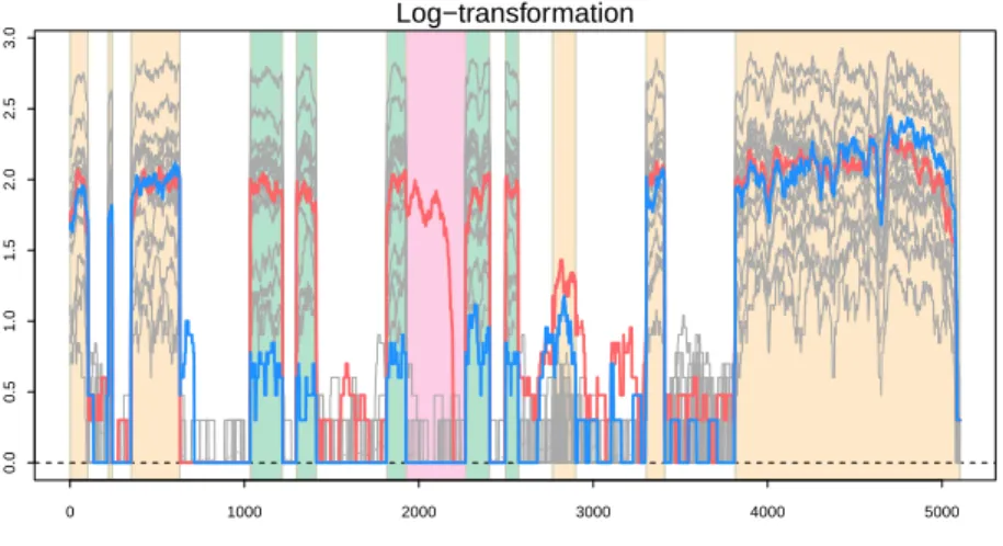
Figure 2.2: The 30 RNA-seq observations for the gene TP53 are plotted on the log-scale. Exons are highlighted by colored background and introns are indicated using mostly white background. The red and blue curves indicate biologically important outliers and the other gray curves indicate normal observations.
The two red and blue outliers show clearly different structure from the other curves, which implies that they show different underlying signals that do not fit together with the majority of the data. At the same time, interestingly, some of the main structures of the two outliers are shared with most of the data. This example motivated us to consider two different types of underlying directions in the data space, together with variation in those directions in describing outliers. Two important types areoutlier directionsthat may lead to prominent high dimensional outliers andmain directionswhose variation is shared among all data points including outliers. The new proposed model incorporating these two components is now introduced in three parts.
Part 1. The classical way of describing underlying variations of a random vector using PCA is discussed in this paragraph. LetX be a random vector distributed as ad-dimensional multivariate normal distribution,Nd(0,ΣΣΣd). The spectral decomposition of the population covariance matrix is
Σ Σ
where Ud = [u1,· · ·,ud] contains the orthonormal eigenvectors of ΣΣΣd in its columns and ΛΛΛd =
diag(λ1,λ2,· · ·,λd)is a diagonal matrix with the corresponding non-negative eigenvalues. Then, a
random vector fromNd(0,ΣΣΣd)can be expressed as
X=UdΛΛΛ
1/2
d Z=UdY
where Z ∼Nd(0,Id) and Y ∼Nd(0,ΛΛΛd). That is, X is a linear combination ofUi with random
coefficientsyifromN(0,λi), i.e.,
X = d
∑
i=1
yiUi, yi∼N(0,λi). (2.3.1)
In the terminology of PCA, the yi are the principal components, i.e. the scores or projection
coefficients (Jolliffe, 2002). Intuitively, ifX involves largeyifor somei, then the directionUiis an
important direction of variation of the underlying distribution ofX, whereas ifyi≈0,X does not feel strongly the directionUi.
Part 2. Distributions for modeling outliers are now considered. Based on the intuition behind the principal components, an outlier can be viewed as an observation that goes strongly in some directions that the bulk of data points do not. Denote one of those directions by Ui∗ and the corresponding random coefficient byy∗i. Then outliers that go in the directionUi∗have largey∗i’s whereas the other data points have smally∗i’s in (2.3.1). We model this underlying variation of a random coefficienty∗i by a scale mixture distribution with two different variances,τi,2τi,1>0, i.e.,
y∗i ∼
√
τi,1zi, w.p. 1−wi
√
τi,2zi, w.p. wi,
(2.3.2)
where the zi’s are i.i.d random variables with mean zero and variance one and 0≤wi≤1, with
distribution with the larger variance,τi,2, corresponds to outliers, and so we assume thatwiis small,
e.g. less than 0.05. This mixture model well reflects an underlying mechanism generating outliers in the sense that “one person’s noise could be another person’s signal”, as pointed out in Kamber and Han (2001).
Part 3. A new model for an underlying distribution embracing a small set of outliers is introduced based on the classical setting (2.3.1) together with the distribution (2.3.2) beyond the Gaussian models. LetX= [X1,· · ·,Xn]be a data matrix whose columns are independent observation vectors
distributed as ad-dimensional (perhaps non-Gaussian) multivariate distribution with a small number of aberrant vectors whose signals are different from the majority of the data. Let{Ui}1≤i≤d be a set of underlying orthogonal vectors some of which are responsible for the potential outliers. Note that these vectors do not need to be the eigenvectors of the underlying covariance matrix. In the spirit of (2.3.1), an observation vectorXjcan be expressed as a linear combination of the orthonormal direction vectors,{Ui}1≤i≤d, whose coefficients are independent random variables distributed as
different mixture distributions, i.e.
Xj= d
∑
i=1
yi jUi, where yi j∼
√
τi,1zi j, w.p. 1−wi
√
τi,2zi j, w.p. wi,
(2.3.3)
where thezi j’s are assumed to be i.i.d. random variables with mean zero, variance one, and bounded
fourth moment. Then, the random variables{yi j}1≤j≤nwithwi>0 model how the directionUias
an outlier component can generate outliers. Also, we will usewi=0 for other directions especially main components, which allows flexibility to include the classical way of describing the variation from underlying directions as in (2.3.1). To distinguish the two components, we letImaindenote a set of dimension indices that correspond to main components andIout denote outlier components. That is, Iout ={1≤i≤d |wi>0}andImain={1≤i≤d |wi=0}={1,· · ·,d}\Iout. Also, we
denote the sample indices that are outlying in each outlier component, indexed by i∈Iout, by
Under the model (2.3.3), outliers are allowed to share important features or background noise with normal data points. The model also allows an outlier to be associated with several outlier components, which offers flexibility in modeling the nature of outliers. Under this setting, a sample vector from (2.3.3) can be viewed as a random vector from a complicated mixture distribution whose components have different covariance structures.
As discussed earlier, still there is no consensus definition for outliers. Every procedure may target its own informal definition for outliers based on various goals. Here, we describe several types of outliers that are commonly used in various applications as special cases of the proposed model in (2.3.3).
• Variable-specific outliers: This type of outlier is different from the bulk of the data only at single variables. If an observation is an outlier with respect to the original variables, then it is usually extreme on these variables. Assuming there ared variables in the model, each sample can be modeled by (2.3.3) withUi=eifor i=1,· · ·,d. Here,ei is a unit vector with 1 for theith entry and 0 for the others. Then, an outlierXjin them-th variable can be described by τm,2>τm,1and an underlying outlier proportionwm.
• Scale mixture outliers: The outliers in this category exhibit a much different abberation, across all variables simultaneously, and are more scattered than the majority of data, and thus they are also known asscatter outliers (Filzmoser et al., 2008). LetXj ∼Nd(0,σ21ΣΣΣ) with probability 1−pand Nd(0,σ22ΣΣΣ)with a small probability pand σ22σ21. This scale mixture model is a special subset of the model (2.3.3) withwi=p,τi,1=σ21,τi,2=σ22 for alli=1,· · ·,d, where theUi’s are a set of the orthogonal vectors, e.g. the eigenvectors ofΣΣΣ. Additionally, theIout will include every index,Imain=0, and/ s1=s2=· · ·=sd. That is,
Xj=
∑di=1yi jUi, where yi j =σ1zi j, w.p. 1−p
• Shifted outliers: The shifted outliers are those that are shifted globally to a common direction (Filzmoser et al., 2008; Ro et al., 2015; Dai and Genton, 2016). Often, these outliers share most of the variation with the the bulk of the data, but present abnormally high or low overall pattern, which is typically described by the mean vector denoted byµ. LetXjbe independent
random vectors fromajµ+Zj, whereZj∼Nd(0,Σ),aj∼N(0,σ21)with probability 1−pand
N(0,σ22)with probability p, andZj andajare independent. Assumingσ1<σ2and a small p, the random variableaj describes how a small fraction of data points may be shifted. Define one of the underlying vectors, sayU1, to be the normalized mean vector, that is,U1=µ/kµk, and the other underlying vectors to be orthogonal to each other. Then, the variation from the U1for normal samples and outliers are respectivelyσ21kµk2+U1TΣΣΣU1andσ22kµk2+U1TΣΣΣU1. Thus, each data object can be modeled by
Xj= d
∑
i=1
yi jUi, where y1j∼
N(0,σ21kµk2+U1TΣΣΣU1), w.p. 1−p N(0,σ22kµk2+U1TΣΣΣU1), w.p. p,
with the otheryi j fromN(0,UiTΣΣΣUi)fori=2,· · ·,d.
2.4 Geometrical representation
It is of great interest to understand when outliers in high dimensions may deviate from the majority and when they may not. Intuitively, ifτi,2in some outlier components are dramatically larger thanτi,1, then the relevant outliers are more likely to be separated from the bulk of the data. By contrast, ifτi,2do not differ much fromτi,1, the corresponding outliers are expected to be harder to distinguish. As discussed below, an interesting observation in high dimensional data is that if an outlier is involved in a large fraction of outlier directions,dencourages the separability of the outlier from the other normal data points even whenτi,2is not substantially large. On the other hand, if an outlier is involved in a limited number of outlier directions,ddiscourages the separability even for relatively largeτi,2’s. We study these phenomena using the geometrical representation of high
dimensional outliers in the HDLSS context explored by Hall et al. (2005) and identify a condition when outliers may be distinguishable in such high dimensions.
We consider a simple scenario where data come from (2.3.3) withτi,1=σ2andτi,2=τ(d)for alliunder the normality assumption. In this section, we index the variation for outlier components byd,τ(d), as an indication of increase with dimension. Then, our model can be expressed as
yi j=
σzi j, w.p. 1−wi τ(d)zi j, w.p. wi,
for i∈Iout and yi j =σzi j fori∈/Iout. (2.4.1)
Consider a non-outlier pointXjfrom (2.4.1) which can be expressed asXj=∑di=1σzi jUiwhere the
Uiare orthonormal underlying eigenvectors. Asdincreases, it follows by a law of large numbers
that its squared Euclidean distance scaled byd converges to the constantσ2in the sense that
1 dkXjk
2 = 1 d
d
∑
i=1 σ2z2i j
→ σ2 (2.4.2)
almost surely. Then, we might fairly say that a non-outlier pointXjlies approximately on the surface
Xlis approximately equal to(2σ2d)1/2asd→∞, in the sense that
1
dkXj−Xlk
2 = 1 d
d
∑
i=1
σ2(zi j−zil)2
→ 2σ2 (2.4.3)
where the convergence is almost sure. These asymptotic results match with the results in Hall et al. (2005). As described in their paper, application of (2.4.3) to each pair(j,l)of non-outliers, and scaling all distances by the factord−1/2, shows that they asymptotically construct a polyhedron where each edge is of length(2σ2)1/2and the vertices are themnon-outliers.
Similarly, we now explore the behavior of outliers in high dimensions. An outlier pointXj0can be expressed as
Xj0 =
∑
i∈Ioutj0 p
τ(d)zi j0Ui+
∑
i∈/Ioutj0σzi j0Ui
whereIoutj0 is an index set for outlier components related toXj0. LetK(d)
j0 =|I j0
out|be the cardinality
of the setIoutj0 for eachdand poutj0 = lim
d→∞ K(jd0)
d be the fraction of the outliers components for a larged.
The deviation ofXj0 from the majority depends on the levels ofK(d)
j0 , that is, p j0
out>0, p j0
out =0 with
K(jd0)→∞, and p
j0
out =0 withK
(d)
j0 fixed. Each case requires the different levels ofτ(d) as will be discussed below.
Let us first consider the case of poutj0 >0 withτ= lim
d→∞
τ(d). It follows that if a law of large numbers applies to its squared distance divided byd, then
1 dkXj0k
2 = 1 d
∑
i∈Ioutj0
τ(d)z2i j0+ 1 d
∑
i∈/Ioutj0
σ2z2i j0
=
K(d)
j0
d 1 K(jd0)
∑
i∈Ioutj0
τ(d)z2i j0+
d−K(d)
j0
d
1 d−K(jd0)
∑
i∈/Ioutj0
σ2z2i j0
→ poutj0 τ+ (1−pj 0
almost surely asd→∞. This implies that an outlier pointXj0 is approximately of distance(σ2d+ poutj0 (τ−σ2)d)1/2 from the origin. Also, the distance between an outlierXj0 and a non-outlierXj
divided byd1/2converges almost surely to(poutj0 (τ−σ2) +2σ2)1/2asd→∞:
1
dkXj−Xj0k
2 = 1 d
∑
i∈Ioutj0
(σzi j−pτ(d)zi j0)2+1 d
∑
i∈/Ioutj0
σ2(zi j−zi j0)2
→ poutj0 (τ−σ2) +2σ2. (2.4.5)
Therefore, a larger poutj0 or a largerτhelp to better separate the outlierXj0 from non-outliers provided
thatτ>σ2andpout >0. In particular, this geometrical property shows that even whenτis not much bigger thanσ2, good separability still follows when pj
0
out is sufficiently large for high dimensions
whereas it tends to be less successful in low dimensions (Filzmoser et al., 2008).
The type of scale mixture outliers introduced in Section 2.3 is a special example of this case withσ21=σ2and σ22=τ. For this particular type, all the resulting outliers have pout=1, which
together with (2.4.2) and (2.4.4) leads to twod-variate spheres of different radii: a sphere of radius
(σ2d)1/2on the surface of which the non-outliers approximately lie, and another sphere of radius
(τd)1/2for the outliers. This geometrical representation is also associated with the unique spectrum limit of the sample covariance matrix of high dimensional scale mixture distributions as studied in Li and Yao (2018). They showed that the limit of the ESD from the scale mixture distribution can be viewed as a mix of the two separate ESD limits relevant to each mixture component, and the separation of these two limits becomes more distinct for a larger ratio of dn. Roughly speaking, the part of the spectrum limit containing large eigenvalues is associated with the larger sphere of radius(τd)1/2and the other part involving smaller eigenvalues is associated with a smaller sphere of radius(σ2d)1/2.
So far, we have observed that d encourages the geometrical separability of an outlier Xj0 if poutj0 >0. However, this is no longer the case forpoutj0 =0 because the termspoutj0 τand pj
0
out(τ−σ2)
separability. So here we letτ(d)increase asdincreases. As mentioned earlier, the case withpj 0
out=0
is further divided into two cases whereK(jd0)increases asd increases and whereK
(d)
j0 is fixed. Let us
first explore the case with increasingK(d)
j0 . We model the idea of a stronger outlier as
K(d)
j0 τ
(d)
d →rj0 asd→∞. (2.4.6)
Then, it is easy to show 1dkXj0k2→rj0+σ2and 1
dkXj−Xj0k
2→r
j0+2σ2asd→∞. This indicates
thatrj0 plays an important role in separatingXj0 from non-outliers geometrically. Ifrj0 is too small, and in particular if it equals 0, then the data points in the sample including outliers asymptotically behave as a regular data set with the absence of outliers. On the other hand, if therj0is large enough, the outlierXj0tends to be distinguished from the sphere on the surface of which the majority of data points spread out.
The results above hold for increasing K(jd0) as d →∞, for fixed sample size n. For the case of a limited number of outlier directions, i.e. K(jd0) =Kj0, a law of large numbers may not be
applicable, and rather we employ the convergence in distribution. Then, we have d1kXj0k2 →d 1
Kj0∑i∈Ioutj0 rj0z 2
i j0+σ
2and 1
dkXj−Xj0k
2→
d K1 j0 ∑i∈Ij
0
out
rj0z2
i j0+2σ
2. Still, we see that the level ofr
j0
determines the separability of an outlier from the other normal data points. But here it is good to mention thatrj0becomes the limit of τ
(d)
d , which only depends on the level ofτ
(d), because we fix
theKj0.
To sum up, our study in this section enables understanding of the transition phenomenon of high dimensional outliers from near the surface of a high dimensional sphere to being distant from the sphere. Our results indicate that there are two factors affecting this transition which are the proportion of outlier components involved in an outlier and the signals of those outlier directions.
2.5 PCA consistency
population eigenvalues are consistently estimated by PCA under some conditions that depend on various asymptotic domains (Shen et al., 2016). We employ the same concept of a spike covariance model here. Let K be the total number of different spike components among the covariance matrices in the mixture components. For convenience, we refer to{Ui}1≤i≤K asspike directionsand
{Ui}K+1≤i≤dasnon-spike directions. The non-spike components are often considered as noise. In a
modification of the definition in Section 2.3, denote the index sets for outlier spike components and main spike components byIout={1≤i≤K|wi>0}andImain={1,· · ·,K}\Iout, respectively. That
is,{Ui}i∈Iout is the set of outlier spike directions and{Ui}i∈Imain is the set of main spike directions.
The inherent variation derived in each directionUican be expressed asλi= (1−wi)τi,1+wiτi,2by the mixture distribution in (2.3.3) and suchλi’s are indeed the population eigenvalues corresponding
to the directionUi. This is because the covariance matrix of Xj from (2.3.3) can be written as
Σ
ΣΣ=Cov(Xj) =Cov(Uyj) =UCov(yj)UT whereyj= (y1j,· · ·,yd j)T. Due to the independence of
{yi j}1≤i≤d, Cov(yj)is a diagonal matrix whose entries arevar(yi j) = (1−wi)τi,1+wiτi,2, and thus theλi’s are the eigenvalues ofΣΣΣby the eigenvalue decomposition.
LetX1,· · ·,Xnbe observations from (2.3.3) with theKspike components as described above. Denote the sample covariance matrix by ˆΣΣΣ=1nXXT =n1∑nj=1XjXTj and its eigenvalue
decomposi-tion by ˆΣΣΣ=UˆΛΛΛˆUˆT with ˆU= [Uˆ1,· · ·,Uˆd]and ˆΛΛΛ=diag(λ1ˆ ,· · ·,λˆd)where{(λˆk,Uˆk):k=1,· · ·,d}
are the pairs of eigenvalues and eigenvectors of ˆΣΣΣsuch that ˆλ1≥λ2ˆ ≥ · · · ≥λˆd. In this section,
asymptotic properties of ˆλ1,· · ·,λˆd and ˆU1,· · ·,Uˆd are analyzed under the general framework
We consider increasing sample sizen, increasing dimensiond, and increasing spike signals. As an indication of increasing spike signals, we let λi,τi,1, andτi,2 be sequences indexed by n, that is,λ(in),τ(i,n1), andτi(,n2). Consider theM+1 tiers where the firstK eigenvalues,{λi(n)}1≤i≤K, are
grouped such that qm eigenvalues fall into the m-th tier where ∑Mm=1qm=K and the rest of the
eigenvalues are all grouped into theM+1-th tier. Defineq0=0,qM+1=d−K, and the partial sums pm=∑ml=0ql. Then, the index set of the eigenvalues in them-th tier can be written as
Hm=pm−1+1,pm−1+2,· · ·,pm−1+qm for m=1,· · ·,M+1.
Denote a linear subspace spanned by the components in them-th tier bySm=span{Ui,i∈Hm}for
m=1,· · ·,M+1.
The following assumptions provide the conditions for the variances, τ(i,n1) and τ(i,n2), of the underlying mixtures. Several different conditions are assumed for main spike signals, outlier spike signals, and noise signals, which helps to distinguish spike components from non-spike components. There are two types of noise in our model. One type is noise for all data points that correspond to the non-spike components in the model. By contrast, the other type is noise for the majority but a signal for a few observations. The latter type of noise is modeled by the small variance part in the outlier components. The following two assumptions illustrate the variances for these two types of noise.
Assumption 2.5.1. lim
n→∞τ
(n)
i,1 =nlim→∞τ
(n)
i,2 =cλ for i∈HM+1.
Assumption 2.5.2. lim
n→∞τ
(n)
i,1 =cλ for i∈Iout.
the Tracy-Widom distribution (Marˇcenko and Pastur, 1967; Bai and Yin, 1988; Bai et al., 1988; Bai and Yin, 1993; Johnstone, 2001). In the same spirit, Assumption 2.5.1 describes the asymptotically equivalent noise signals for non-spike directions{Ui}i∈HM+1. Eventually, the underlying eigenvalues
{λ(in)}i>K are all equal tocλ for larged. Assumption 2.5.2 describes noise variances (τ
(n)
i,1) for the outlier spike components. Since the outlier spike components are nothing but noise for the majority of the data, the same level of variation assumed for the non-spike components can be assumed. Thus, the noise variances for outlier spike directions are also asymptotically equal tocλ. This nicely connects the outlier model with the null model, i.e. the case with no outlier spike components, in the sense that the outlier components will merge with non-spike noise components.
In contrast to noise signals, we allow spike signals to be increasing inn. The intensity of each spike component is determined by the underlying variation that each component is involved in, which is equivalent to its corresponding eigenvalue. For largen, the underlying eigenvalues,λ(in), are simplyτ(i,n1)fori∈Imainwhereas, fori∈Iout, the eigenvalues arewiτ
(n)
i,2 because variation from the larger variance componentτ(i,n2) dominate variation from the smaller variance componentτ(i,n1). The PCA consistency strongly depends on the magnitudes of spike eigenvalues, which are specified in a systematic manner in the following assumptions. Letδ(mn) for m=1,· · ·,Mbe sequences of
constant values for indexn. Assumption 2.5.3. lim
n→∞ τ(i,n1)
δ(mn)
=1for i∈Hm∩Imainand lim n→∞
τ(i,n2)
wiδ(mn)
=1for i∈Hm∩Iout, m=1,· · ·,M.
Assumption 2.5.4. As n→∞,δ(1n)δ(2n) · · · δM(n)λ(Kn+)1where anbnimplies lim n→∞
an bn >1.
Assumption 2.5.3 allows the components in the same tier to share asymptotically equivalent eigenvalues. We further assume different limiting coefficients for different tiers in Assumption 2.5.4, which enables the characterization of theMsubspaces spanned by the directions in each tier.
they are allowed to share the same underlying eigenvectors from the model (2.3.3). Then, we have a simple integrated covariance matrixΣΣΣso that a spike covariance model can be employed even when data come from multiple distributions.
In general, the strength of underlying spike signals and increasing sample sizenencourage PCA consistency whereas increasing dimensionddiscourages consistency. When the underlying spike signals in them-th tier with increasingnare asymptotically strong enough to prevail over the dimensiondin the sense that d
nδ(mn)
→0, it follows that the estimates of the eigenvectors are subspace consistent in them-th tier and the estimates of the eigenvalues are consistent as well. Theorems 2.5.1 and 2.5.2 demonstrate such asymptotic behavior in a concrete manner under different scenarios. Theorem 2.5.1. Under Assumptions 2.5.1-2.5.4,
(a) if d
nδ(Mn) →0, then
(i) for i≤K, ˆλi λ(in)
→a.s.1whereλi(n)=τ(i,n1) for i∈Imainandλ(in)=wiτi(,n2) for i∈Iout;
(ii) for i>K,
• if0<c<∞, cλ(1−√c)2≤λˆn∧d≤λˆ1≤cλ(1+
√
c)2a.s.; • if c=∞, nˆλi
d →a.s.cλ;
• if c=0,ˆλi→a.s.cλ;
(b) if d
nδ(hn) →0where1≤h<M and d
nδ(hn+)1 →∞, then
(i) for i≤ph, ˆλi λ(in)
→a.s.1whereλi(n)=τ(i,n1) for i∈Imainandλ(in)=wiτi(,n2)for i∈Iout;
(ii) for i>ph, nλˆi
d →a.s.cλ.
Theorem 2.5.1 considers two scenarios: (a) when all spike signals are strong and (b) when strong population signals are assumed only up to theh-th tier and the other signals are dominated by the increasing dimension, i.e. d
nδ(hn+)1 →∞. It should be noted that these two different scenarios
condition d
nδ(hn+)1 →∞of (b) and Assumption 2.5.4 together rule out the cases ofc<∞as d
nλ(Kn+)1 →∞
can hold only when dn→∞. In both cases, if the signal in a tier is strong enough so that d
nδ(n) →0,
then the sample eigenvalues corresponding to the tier consistently estimate the true eigenvalues. On the other hand, if the spike signals are not that strong, then the corresponding sample eigenvalues tend to be swallowed by the small bulk eigenvalues.
Intuitively, although an underlying outlier component is dramatically intense, its realized signal is much weaker than the true one because it loses the power due to the small chance of participation. Assumption 2.5.3 reflects this intuition and gives a condition that theith outlier spike signal should be 1/witimes greater than the other main spike signals in the same tier to compensate for this loss of power. Based on this assumption, Theorem 2.5.1 demonstrates that such an outlier signal would asymptotically attain the same sample eigenvalues as the main signals in the same tier. In particular, the sample eigenvalue from an outlier signal converges to the dominating variance (τ(i,n2)) multiplied by the corresponding proportion (wi) in the underlying mixture distribution (2.3.3). Therefore,
the true levels of outlier signals can be approximately estimated by dividing the corresponding eigenvalues by the proportion (≈wi) of the relevant outliers.
In many outlier detection methods, it is of great interest to choose the subspace that outlier components are involved in (Filzmoser et al., 2008; Ahn et al., 2018). Although Theorem 2.5.1 suggests that a few large sample eigenvalues may consistently estimate the true levels of the signals, it is not enough to say that the corresponding principal component directions construct a useful subspace for detecting outliers. This brings to the study of eigenvectors that is discussed in the following theorem. Letδ(0n)=∞for alln.
Theorem 2.5.2. Under Assumptions 2.5.1-2.5.4,
(a) if d
nδ(Mn) →0, and0<c≤∞, then
(i) Uˆiare subspace consistent in the sense that theangle(Uˆi,Sm)→a.s.0for i∈Hm, m=
1,· · ·,M+1.
• For m=1,· · ·,M−1,angle(Uˆi,Sm) =o( δ(mn) δ(mn−)1
∨δ
(n)
m+1
δ(mn)
1/2
• For m=M,angle(Uˆi,Sm) =o( δ(mn) δ(mn−)1
1/2
)∨O( d nδ(mn)
1/2
). • For m=M+1,angle(Uˆi,Sm) =O( d
nδ(mn−)1
1/2
).
(b) if d
nδ(hn) →0where1≤h<M and d
nδ(hn+)1 →∞, then
(i) Uˆi for i≤ ph are subspace consistent in the sense that the angle(Uˆi,Sm)→a.s. 0 for
i∈Hm, m=1,· · ·,h.
• For m=1,· · ·,h−1,angle(Uˆi,Sm) =o( δ(mn) δ(mn−)1
∨δ
(n)
m+1
δ(mn)
1/2
). • For m=h,angle(Uˆi,Sm) =o(
δ(mn)
δ(mn−)1
1/2
)∨O( d nδ(mn)
1/2
).
(ii) Uˆifor i> phare strongly inconsistent in the sense that|<Uˆi,Ui>|=O( nλ(in)
d
1/2
).
Under the same scenarios considered in Theorem 2.5.1, Theorem 2.5.2 studies the asymptotic behavior of the sample eigenvectors in terms of angles as studied in Jung and Marron (2009) and Shen et al. (2016). In each scenario, if themth tier involves a strong signal such that d
nδ(mn)
→0, then theith sample eigenvector, ˆUifori∈Hm, tends to be in the subspace,Sm, which is spanned by the
underlying directions in themth tier. This holds for alli∈Hm, and thus it follows that the subspace
spanned by the sample eigenvectors,{Uˆi}i∈H
m, converges to theSm. This phenomenon is called
the PCA subspace consistency. Also, the different levels of signals in different tiers assumed in Assumption 2.5.4 make the estimated subspaces become distinct for largenand larged, and more gaps between the levels accelerate this distinction as indicated by the different convergence rates obtained in the theorem.
the outlier-relevant low dimensional subspace by using the first few PC directions whose sample eigenvalues are substantially large and thus separate from the other bulk eigenvalues.
On the other hand, Theorem 2.5.2 (b) together with Theorem 2.5.1 (b) shows that when only a subset of the outlier signals are strong enough to dominate the increasing dimensions, the first few PC directions with large sample eigenvalues provide a good subspace only for those strong outlier components. Not only this, the strong inconsistency suggests that it becomes very challenging to distinguish the outlier directions missing from the first few PCs from the non-spike directions. This is not simply because the sample eigenvalues from those weak outlier signals are not separable from the bulk sample eigenvalues. Once the spike samples eigenvalues are swallowed by the bulk, then it is likely that the corresponding directions are all mixed with non-spike directions, so any of the single sample eigenvectors may not be representative of those spike directions. Therefore, the approximation of the data matrix using the first few eigenvectors may miss some important information that are relatively weak but not noise. This implies that the outlier components with weak signals or with extremely small participation are harder to be separated from noise. Thus special care should be taken to find the hidden outlying structure.
Also, it should be noted that the theorem does not guarantee that the sample eigenvectors are individually consistent to the true ones. So looking at the individual PC directions may not be enough to detect outliers. To illustrate this situation, a toy example is given in Section 2.6. As one of the special and important cases, we now consider the case when all spike eigenvalues are separable,
i.e.q1=q2=· · ·=qM=1 andM=K. Then, Assumption 2.5.4 becomes
Assumption 2.5.5. As n→∞,λ(1n)λ(2n) · · · λ(Kn)λ(Kn+)1>0.
This allows us to get the individual consistency of eigenvalues as well as eigenvectors instead of subspace consistency. The following corollaries of Theorem 2.5.1 and 2.5.2 describe such individual consistency under the same scenarios with the respective theorems.
Corollary 2.5.1. Under Assumptions 2.5.1, 2.5.2, and 2.5.5, (a) if d
(i) for i≤K, ˆλi λ(in)
→a.s.1whereλi(n)=τ(i,n1) for i∈Imainandλ(in)=wiτi(,n2) for i∈Iout;
(ii) for i>K,
• if0<c<∞, cλ(1−√c)2≤λˆn∧d≤λˆ1≤cλ(1+
√
c)2a.s.; • if c=∞, nˆλi
d →a.s.cλ;
• if c=0,ˆλi→a.s.cλ;
(b) if d
nλ(hn) →0where1≤h<K and d
nλ(hn+)1 →∞, then
(i) for i≤h, ˆλi λ(in)
→a.s.1whereλi(n)=τ(i,n1) for i∈Imainandλ(in)=wiτi(,n2) for i∈Iout;
(ii) for i>h, nλˆi
d →a.s.cλ.
Corollary 2.5.2. Under Assumptions 2.5.1, 2.5.2, and 2.5.5,
(a) if d
nλ(Kn) →0, and0<c≤∞, then
(i) Uˆiare consistent with Uiin the sense thatangle(Uˆi,Ui)→a.s.0for i=1,· · ·,K.
• For i=1,· · ·,K−1,angle(Uˆi,Ui) =o( λ(in)
λ(i−n)1
∨λ
(n)
i+1
λ(in)
1/2
). • For i=K,angle(Uˆi,Ui) =o(
λ(in)
λ(i−n)1
1/2
)∨O( d nλ(in)
1/2
). • For i>K,angle(Uˆi,S) =O( d
nλ(i−n)1
1/2
)where S=span(Ui:i>K).
(b) if d
nλ(hn) →0where1≤h<K and d
nλ(hn+)1 →∞, then
(i) Uˆiare consistent with Uiin the sense thatangle(Uˆi,Ui)→a.s.0for i=1,· · ·,h.
• For i=1,· · ·,h−1,angle(Uˆi,Ui) =o( λ(in)
λ(i−n)1
∨λ
(n)
i+1
λ(mn)
1/2
). • For i=h,angle(Uˆi,Ui) =o(
λ(in)
λ(i−n)1
1/2
)∨O( d nλ(in)
1/2
).
(ii) Uˆifor i>h are strongly inconsistent in the sense that|<Uˆi,Ui>|=O( nλ(in)
d
1/2
2.6 Illustration using a toy example
We now illustrate the PCA subspace consistency with a toy example under the model (2.3.3), highlighting the situation where an outlier component is captured by the first few PC directions but none of the PC directions are individually representative of the outlier component.
First, let us describe the simulation setting. We generated n=200 independent data vec-tors in d =3000 dimensions based on our model described in (2.3.3). To generate such data, {zi j}1≤i≤d,1≤j≤nare assumed to be distributed as independentN(0,1)and the standard basis vec-tors,{ei}1≤i≤d, are used as underlying eigenvectors{Ui}1≤i≤d withe1,· · ·,e9being the main spike directions ande10 being an outlier spike direction. For the main spike directions, the underlying variations are assumed to beτi,1=3000,1000,100,90,80,70,60,50,40 fori=1,· · ·,9. For the outlier spike directione10, we assumeτ10,1=2000,τ10,2=1 and the outlier proportionw10=0.02. For the other non-spike directions {Ui}11≤i≤d corresponding to noise, τi,1=1 and τi,2=1 are assumed. A realization from this model had the 4 outliers, denoted byX1,· · ·,X4, with 196 normal data points, denoted byX5,· · ·,X200.
For this data set, we constructed a sample covariance matrix where PCA was applied and obtained a set of sample eigenvectors and eigenvalues. Since the true spike directions aree1,· · ·,e10, we can examine the contribution of each sample eigenvector onto the true spike directions simply by taking the squares of the entries. The sum of the squares of entries in each sample eigenvector is one and thus the squared values ˆu2ji, i.e. the squared jth entry of ˆUi, can be regarded as the explained percentage of the underlying vectorejin the direction ˆUi. Table 2.1 gives the squares of the first 12 entries (in rows) of the first 11 eigenvectors ˆU1,· · ·,Uˆ11 (in columns). The last two rows indicate the corresponding sample eigenvalues ˆλiand the angles between the true outlier directione10 and
ˆ
Uifori=1,· · ·,11. The largest value in each ˆUiis indicated using red, and if the red value, say ˆu2ji,
is close to one and the other entries are close to zero, then the ˆUiis a good estimate of theej. For
On the other hand, none of the ˆU3,· · ·,Uˆ10 has an entry which is close to one. Instead, they have several nonzero entries, indicating that each of them has some correlation with several underlying directions. This can be understood that any of the underlying directions,e3,· · ·,e10 are well estimated by the single sample eigenvectors. Nonetheless, an important note is that, for each row j=3,· · ·,10, the sum of the squared jth entries of ˆU3,· · ·,Uˆ10is close to one. This supports the PCA subspace consistency in that each of the true eigenvectorse3,· · ·,e10 can be estimated by a linear combination of ˆU3,· · ·,Uˆ10 rather than any individual directions. As described in Theorem 2.5.2, this is because the underlying variation ine3,· · ·,e10 are nearly in the same tier, which tends to somewhat discourage the individual consistency.
ˆ
U1 Uˆ2 Uˆ3 Uˆ4 Uˆ5 Uˆ6 Uˆ7 Uˆ8 Uˆ9 Uˆ10 Uˆ11
1 0.996 0.000 0.000 0.000 0.000 0.000 0.000 0.000 0.000 0.000 0.000
2 0.000 0.987 0.000 0.000 0.000 0.000 0.000 0.000 0.001 0.000 0.000 3 0.000 0.000 0.657 0.001 0.072 0.173 0.004 0.000 0.000 0.002 0.000 4 0.000 0.000 0.020 0.665 0.111 0.023 0.055 0.011 0.001 0.003 0.000 5 0.000 0.001 0.029 0.031 0.330 0.422 0.048 0.008 0.001 0.013 0.000 6 0.000 0.000 0.071 0.006 0.198 0.023 0.064 0.501 0.007 0.003 0.000 7 0.000 0.000 0.036 0.002 0.080 0.009 0.408 0.201 0.053 0.059 0.000 8 0.000 0.000 0.000 0.007 0.004 0.021 0.094 0.047 0.243 0.382 0.000 9 0.000 0.001 0.003 0.000 0.012 0.001 0.010 0.000 0.467 0.292 0.000 10 0.000 0.000 0.101 0.182 0.079 0.215 0.169 0.096 0.030 0.007 0.000 11 0.000 0.000 0.000 0.000 0.000 0.000 0.000 0.000 0.000 0.000 0.000 12 0.000 0.000 0.000 0.000 0.000 0.000 0.000 0.000 0.000 0.000 0.000
..
. ... ... ... ... ... ... ... ... ... ... ˆ
λi 3519.209 996.408 123.856 99.055 91.825 86.694 71.458 70.393 52.236 42.087 16.850
angle 89.6 89.1 71.5 64.8 73.7 62.4 65.7 71.9 80.0 85.3 89.4
Table 2.1:This table shows the first 11 sample eigenvectors with squared entries. The largest value in each ˆUiis colored using a red font and the row
corresponding to the outlier signal,e10, is hightlighted using lightblue background. This row indicates how much each ˆUiexplains the outlier signal.
The last two rows respectively show the sample eigenvalues corresponding to{Uˆi}1≤i≤11and the angles between ˆUi and the true outlier signal,e10.
2.7 Proofs
In this section, we provide proofs for the theorems in Section 2.5. The main steps in the proofs are similar to the proofs in Shen et al. (2016) but our different setting for the underlying distribution of data requires the addition of more detail.
LetYbe ad×nmatrix whose column vectors areY1,Y2,· · ·,YnwhereYj= (y1j,· · ·,yd j)T and
yi j’s are independent random variables in our model in (2.3.3). Then, switching the roles of columns and rows, we get then×ndual (Gram) matrix of the sample covariance matrix ˆΣΣΣ
ˆ ΣΣΣD=
1 nX
TX= 1
nY
TUTUY=1
nY
TY,
and it is well known that they share the same nonzero eigenvalues. Let us define two matrices that will be treated separately in the proof. Let
A= 1
n
K
∑
i=1 ˜
YiY˜iT, and B=1
n
d
∑
i=K+1 ˜ YiY˜iT,
where ˜Yiis thei-th row vector ofY. Then,
ˆ ΣΣΣD =
1 n
d
∑
i=1 ˜
YiY˜iT =A+B.
Before the proof, we provide two popular lemmas. Lemma 2.7.1 provides the upper and lower bounds for the eigenvalues of a matrix that can be expressed as the sum of two symmetric matrices. Lemma 2.7.1. (Weyl inequality) Let A and B be n×n real symmetric matrices. Then, for all
j,k,l=1,· · ·,n,
λk(A) +λl(B) ≤ λj(A+B) fork+l= j+n
whereλj(A)is the j-th largest eigenvalue of a matrix A.
Next, Lemma 2.7.2 provides the convergence of the largest and smallest non-zero eigenvalues of a random matrix, which is known as Bai-Yin’s law (Bai and Yin, 1993).
Lemma 2.7.2. (Bai-Yin’s law) Suppose B= 1qVVT where V is a p×q random matrix composed of i.i.d. random variables with zero mean, unit variance and finite fourth moment. As q→∞ and qp→c∈[0,∞), the largest and smallest non-zero eigenvalues of B converge almost surely to
(1+√c)2and(1−√c)2, respectively.
2.7.1 Proof of Theorem 2.5.1
Proof. The proof consists of the following three steps: 1. Establish the convergence ofλk(A).
2. Establish the convergence ofλk(B).
3. Establish the convergence ofλk(A+B).
Lemma 2.7.3 proves the first step. Lemma 2.7.3. As n→∞, we have
1 λ(kn)
λk(A)→1 a.s. for k=1,· · ·,K.
whereλ(in)=τi(,n1) for i∈Imain andλ(in)=wiτi(,n2)for i∈Iout.
Proof. DefineAk= 1n∑Ki=kY˜iY˜iT withAk,Dbeing its dual matrix andAk,R=A−Ak. Then,
λ1(1 nY˜kY˜
T
k ) +λn(
1 n
K
∑
i=k+1 ˜
YiY˜iT)≤λk(A)≤λ1(Ak) +λk(Ak,R) (2.7.1)