Xie_unc_0153D_15623.pdf

ESTIMATION OF GRAPHICAL MODELS WITH BIOLOGICAL APPLICATIONS

Yuying Xie

A dissertation submitted to the faculty of the University of North Carolina at Chapel Hill

in partial fulfillment of the requirements for the degree of Doctor of Philosophy in the

Department of Statistics and Operations Research.

Chapel Hill

2015

c

2015

Yuying Xie

ABSTRACT

Yuying Xie: ESTIMATION OF GRAPHICAL MODELS WITH BIOLOGICAL

APPLICATIONS

(Under the direction of Yufeng Liu and William Valdar)

Graphical models are widely used to represent the dependency relationship among

ran-dom variables. In this dissertation, we have developed three statistical methodologies for

estimating graphical models using high dimensional genomic data. In the first two, we

estimate undirected Gaussian graphical models (GGMs) which capture the conditional

de-pendence among variables, and in the third, we describe a novel method to estimate a

Gaussian Directed Acyclic Graph (DAG).

In the first project, we focus on estimating GGMs from a group of dependent data.

A motivating example is that of modeling gene expression collected on multiple tissues

from the same individual. Existing methods that assume independence among graphs are

not applicable in this setting. To estimate multiple dependent graphs, we decompose the

problem into two graphical layers: the systemic layer, which is the network affecting all

outcomes and therefore describing cross-graph dependency, and the category-specific layer,

which represents the graph-specific variation. We propose a new graphical EM technique

that estimates the two layers jointly; and also establish the estimation consistency and

selection sparsistency of the proposed estimator. We confirm by simulation and real data

analysis that our EM method is superior to a naive one-step method

study suggests that our method have substantially higher sensitivity and specificity to

esti-mate the underlying graph than existing methods.

ACKNOWLEDGEMENTS

A great many people have helped me throughout my graduate research. I finally finished

the journey to my second and also potentially last Ph.D degree. I owe my gratitude to all

those who gave me direction, instruction, and courage. Thank you very much!

First, I would like to sincerely thank my co-mentor Dr. Yufeng Liu. I am extremely

fortunate to have an advisor who gave me the freedom to explore, and at the same time,

the guidance to recover when I lost confidence in my research. I still remember how excited

and nervous I was when I first talked to Yufeng about the possibility of working with him

for my second Ph.D in Statistics. He taught me, encouraged me, and led me into the area

of statistical machine learning. Without his constant encouragement and support, I would

not have accomplished as much. I value Yufeng’s creativity in developing novel machine

learning methodologies to analyze biological data with complicated structure, and admire

his passion for both work and life. He has been a role model for me as a researcher and a

teacher.

I also would like to thank my other mentor, Dr. William Valdar, for his support, advice,

criticism, and encouragement for the past five years. It was Will who dragged me into a dry

lab. He taught me not only about how to program efficiently, but also about how express

ideas clearly. Most importantly, he taught me how to question thoughts and progress a

topic beyond its current understanding. It has been a pleasure and great honor to be your

student.

professor who to sit on the committees of both my Ph.D.s. He greatly cares for his students,

even letting me borrow his office for my phone interviews. He gave me great suggestions

for my project and was always willing to shared his code.

Amazing lab members and classmates were another treasure I got during my study. We

went through all the up and down together. I greatly value their friendship and I deeply

appreciate their belief in me. I have to give a special mention for the support given by Dr.

Allen Larnacic, Dr. Zhaojun Zhang, Dr. Jeremy Sabourin, Dr. Wonyul Lee, Dr. Qiang

Sun, Dr. Chang Zhang, Dr. Guanhua Chen, Dr. Sunyoung Shin, Dr. Patrick Kimes, Guan

Yu, Daniel Oreper, Greg Keele, Dr Jeff Roach, Paul Maurizio, and Robert Corty.

TABLE OF CONTENTS

LIST OF TABLES . . . .

x

LIST OF FIGURES . . . .

xi

1

Introduction . . . .

1

1.1

Gaussian Graphical Models . . . .

2

1.2

Extensions of Gaussian Graphical Models . . . .

3

1.3

Bayesian Networks and Directed Acyclic Graphs . . . .

4

1.4

Estimation of Directed Acyclic Graphs and Skeleton . . . .

5

2

Joint Estimation of Multiple Dependent Gaussian Graphical Models with

Applications to Mouse Genomics . . . .

7

2.1

Introduction

. . . .

7

2.2

Methodology . . . .

11

2.2.1

Problem formulation . . . .

12

2.2.2

One-step method . . . .

13

2.2.3

Graphical EM method . . . .

14

2.2.4

Model selection . . . .

17

2.3

Asymptotic properties . . . .

18

2.4

Simulation . . . .

20

2.4.1

Simulating category-specific and systemic networks . . . .

21

2.4.2

Criteria for evaluating performance . . . .

22

2.4.3

Estimation of category-specific Ω

k

and systemic networks Ω

0

. . . .

22

2.4.4

Estimation of aggregate networks ΩY

k

. . . .

25

2.5

Application to gene expression data in mouse . . . .

25

2.7

Appendix . . . .

35

2.7.1

Derivation of likelihood for y . . . .

35

2.7.2

Proof of Identifiability . . . .

37

2.7.3

Proof of Proposition 2.1 . . . .

39

2.7.4

Proof of Theorem 2.1 . . . .

49

2.7.5

Proof of Corollary 2.1 . . . .

53

2.7.6

Proof of Theorem 2.2 . . . .

54

2.7.7

Proof of Theorem 2.3 . . . .

59

2.7.8

Proof of Theorem 2.4 . . . .

61

2.7.9

Extension with Similarity Parameter

α

k

. . . .

61

3

Estimation of Gaussian Graphical Model from Data with Dependent

Noise Structure . . . .

67

3.1

Introduction . . . .

67

3.2

Methodology . . . .

71

3.2.1

Problem formulation . . . .

71

3.2.2

One-step method . . . .

72

3.2.3

Graphical EM method . . . .

74

3.3

Asymptotic properties . . . .

76

3.4

Numerical Example . . . .

78

3.4.1

Simulating

X

and

networks . . . .

79

3.5

Discussion . . . .

83

3.6

Appendix . . . .

83

3.6.1

Derivation of likelihood for y . . . .

83

3.6.2

Proof of Identifiability . . . .

84

3.6.3

Proof of Corollary 3.1 . . . .

85

4

Estimation of the Skeletons in High Dimensional Directed Acyclic Graphs

using Adaptive Group Lasso . . . .

86

4.2

Preliminaries . . . .

89

4.2.1

Definition and Terminology for DAG . . . .

89

4.2.2

Gaussian Graphical Model and Correlation Graph . . . .

90

4.3

Methodology . . . .

92

4.3.1

Problem Formulation . . . .

92

4.3.2

The AdaPC Algorithm . . . .

93

4.4

Simulation Examples . . . .

95

4.4.1

Simulating set-up . . . .

96

4.4.2

Relationship between

M

and skeleton . . . .

97

4.4.3

Estimation of

M

. . . .

98

4.4.4

Estimation of the Skeleton . . . .

99

4.5

Application . . . .

99

4.6

Discussion . . . 102

LIST OF TABLES

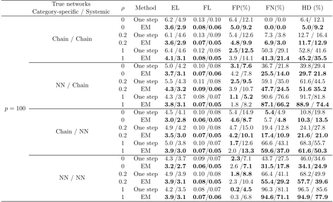
2.1

Summary statistics reporting performance of the EM and one-step

methods inferring graph structure for different networks. In each

cell, the number before and after the slash correspond to the results

using extended BIC and cross-validation, respectively. . . .

31

2.2

Summary statistics reporting performance of the EM and one-step

methods inferring graph structure for different networks. In each

cell, the number before and after the slash correspond to the results

using extended BIC and cross-validation, respectively. . . .

32

2.3

Summary statistics reporting performance of HL, JGL, one-step and

the EM methods estimating aggregate network ,ΩY

, under different

simulation settings with dimension

p

= 30 and 100. . . .

33

3.1

Summary statistics reporting performance of the EM and one-step

methods inferring graph structure for different networks. In each

cell, the number before and after the slash correspond to the results

using extended BIC and cross-validation, respectively. . . .

81

3.2

Summary statistics reporting performance of the EM and one-step

methods inferring graph structure for different networks. In each

cell, the number before and after the slash correspond to the results

LIST OF FIGURES

2.1

Illustration of systemic and category-specific networks using a toy

example with two categories (C1 and

C2) and

p

= 10 variables.

a) Category-specific network for

C1. b) Category-specific network

for

C2. c) Systemic network affecting variables in both

C

1

and

C

2

.

d)Aggregate network, Ω

Y1

= (Ω

−1

1

+ Ω

−1 0

)

−1

_{, for category}

_C

1

. e)

Aggregate network, Ω

Y2

= (Ω

−1 2

+ Ω

−1

0

)

−1

, for

C

2

. . . .

11

2.2

Network topologies generated in the simulations. Top row (a-c)

shows chain networks with noise ratios

ρ

= 0, 0.2, and 1. Bottom

row (d-e) shows nearest-neighbor (NN) networks with

ρ

= 0, 0.2,

and 1. . . .

20

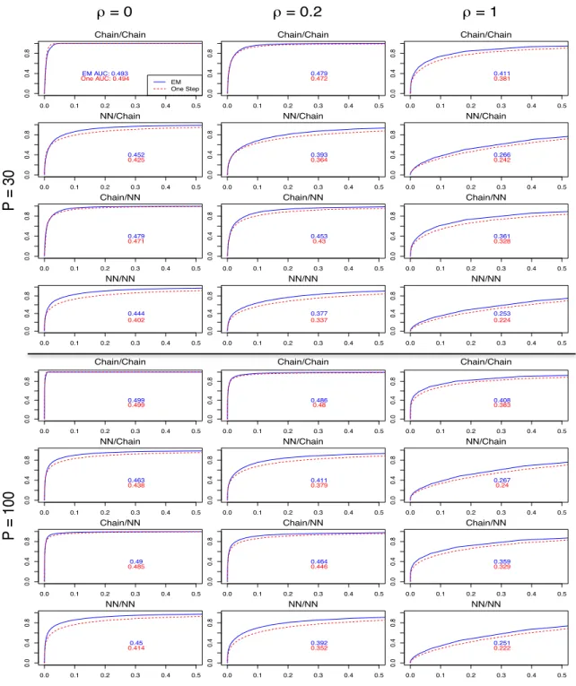
2.3

Receiver operating characteristic (ROC) curves assessing power and

discrimination of graphical inference under different simulation

set-tings. Each panel reports performance of the EM method (blue

line) and the one-step method (dashed line), plotting true positive

rate (y-axis) against false positive rate (x-axis) for a given noise ratio

ρ. . . .

24

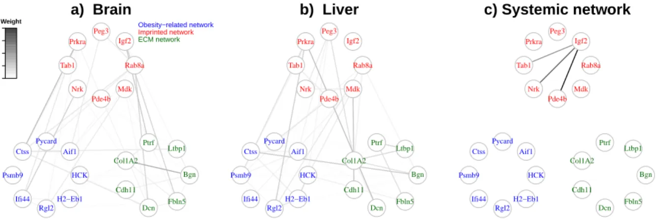
2.4

Topology of gene co-expression networks inferred by the

EM-method for the data from a population of F

2

mice with randomly

allocated high-fat vs normal gene variants. Panels a) and b) display

the estimated brain-specific and liver-specific dependency structures

respectively. Panel c) shows the estimated systemic structure

de-scribing whole body interaction that simultaneously affect variables

in both tissues. . . .

28

2.5

Topology of gene co-expression networks inferred by the

EM-method for the data from a population of reciprocal F

1

mice.

Pan-els a) and b) display the estimated brain-specific and liver-specific

dependency structures respectively. Panel c) shows the estimated

systemic structure describing whole body interaction that

simulta-neously affect variables in both tissues. . . .

29

2.6

Topology of co-expression networks inferred by the EM method

ap-plied to measurements of the 1000 genes with highest within-tissue

variance in a population of F

2

mice. Panels a), b), c) and d) display

the category-specific networks estimated for adipose, hypothalamus,

liver and muscle tissues respectively. Panel e) shows the structure

of the estimated systemic network, describing across-tissue

depen-dencies, with panel f) showing a zoomed-in view of the connected

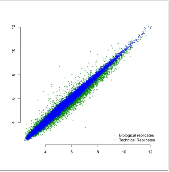
3.1

Effect of measurement error is illustrated through a scatter plot.

Each point represents a gene, X and Y axes are gene expression

levels measured by microarray. Blue dots are technical replicates

that are the same sample measured twice using two different

mi-croarrays. Green dots are biological replicates. A large proportion

of the total variance is due to measurement error. . . .

69

3.2

Effect of measurement error on Ω

Y

with

p

= 10 variables. The left

figures is the true Ω

X

, and the right figure is Ω

Y

= (Ω

−_X1

+ Ω

−1

)

−1

. . . .

70

3.3

Network topologies generated in the simulations. . . .

78

3.4

Receiver operating characteristic (ROC) curves assessing power and

discrimination of graphical inference for

p

= 100 and

n

= 500. Each

panel reports performance of the EM method (blue line) and the

Glasso method (red line), plotting true positive rate (y-axis)against

false positive rate (x-axis) for a given noise ratio. . . .

80

3.5

Receiver operating characteristic (ROC) curves assessing power and

discrimination of graphical inference for

p

∈ {30,

100}

and

n

= 500.

Each panel reports performance of the EM method (blue line) and

the one-step method (green line), plotting true positive rate

(y-axis)against false positive rate (x-axis) for a given noise ratio. . . .

82

4.1

Illustration of the relationship among DAG, skeleton, GGN, CG,

and GGN

∩

CG. . . .

92

4.2

DAG topologies used in the simulations. (a) and (b) shows the

DAG with

E

= 2 and 5 respectively. . . .

96

4.3

Illustration of the relationship between graph

M

and skeleton. Each

panel plots the Ω value (x-axis) against the Σ value (y-axis) with

red dots representing those entries with edges in the skeleton, while

blue dots representing entries without edges. . . .

97

4.4

Receiver operating characteristic (ROC) curve for estimating

M.

Each panel reports the performance of the AdaPC method (blue

line) and the separate method (orange, grey, yellow and brown lines

represent the fixed

λ

3

for a given sparsity parameter

E. . . .

98

4.5

ROC curve assessing power and discrimination of estimating the

skeleton of a DAG. The blue solid line represents the AdaPC

algo-rithm and dash red line is result from PC-stable algoalgo-rithm. . . .

99

4.6

Topology of the skeleton networks inferred by the EM method

applied to measurements of the 394 genes with highest

within-tissue variance in Mesenchymal subclass. Panels a) and b) display

the skeleton networks estimated by AdaPC method and PC-stable

CHAPTER 1

Introduction

With the advance of technology in recent years, we have witnessed a data explosion

in many fields including biological science, social network and engineering. As a result, in

order to better explore and understand the information behind large and maybe noisy data

sets, there is a great need for the development of new statistical methodologies. A graphical

model is a probabilistic model which uses a graph to denote the conditional dependence

structure among random variables. Since graphs are conveniently used to provide insight

and capture complex dependencies among random variables, graphical models have become

an important focus of research in recent years. For example, in biological research, genes

can be represented by the nodes of a graph, and the correlations between genes can be

represented by the edges. In the area of finance, nodes of a graph can represent different

stocks in Nasdaq and edges can represent the partial correlation between stocks.

1.1

Gaussian Graphical Models

Gaussian Graphical models (GGMs) are widely used to represent conditional

depen-dencies among sets of normally distributed outcome variables that are observed together.

For example, observed, and potentially dense, correlations between measurements of

ex-pression for multiple genes, stock market prices of different asset classes, or blood flow for

multiple voxels in functional Magnetic Resonance Imaging (fMRI)-measured brain activity

can often be more parsimoniously explained by an underlying graph corresponding to the

partial correlation. The partial correlation matrix is normally assumed to be sparse, since

most of the time two variables interact with each other through other variables, hence the

partial correlation between these two variables given all other variables is zero. As methods

for estimating these underlying graphs have matured, a number of elaborations to the basic

GGM have been proposed; these include elaborations that seek either to model more closely

the sampling distribution of the data, or to model prior expectations of the analyst about

structural similarities among graphs representing data sets that are related.

Introduced more formally, the conditional dependence relationships among a set of

p

outcome variables,

y

= (y

1

, ..., yp), can be represented by a graph

G

= (X, E) where each

variable corresponds to a node in the set

V

and conditional dependencies are represented

by the edges in the set

E. If we further assume that the joint distribution of the outcome

variables is multivariate Gaussian,

y

∼ N

(0,

Σ), then conditional dependencies are reflected

in the non-zero entries of the precision matrix Ω = Σ

−1

. Specifically, variables

i

and

j

are

conditionally independent given the other variables if and only if the (i, j)-th element of

Ω is zero. Inferring the dependence structure of such a Gaussian graphical model is thus

equivalent to estimating which elements of its precision matrix are non-zero.

to determine iteratively the edges of each node in

G

by regressing the corresponding variable

yj

on the remaining variables

y

−j

under an

`

1

penalty, an approach which can be viewed

as optimizing a pseudo-likelihood (Rocha et al., 2008; Ambroise et al., 2009; Peng et al.,

2009). Several groups have proposed sparse penalized maximum likelihood to estimate

GGMs(see for example Yuan and Lin, 2007; Banerjee et al., 2008; d’Aspremont et al., 2008;

Rothman et al., 2008). Several efficient implementations solving this problem have also been

published including the graphical-LASSO (GLASSO) algorithm (Friedman et al., 2008) and

the QUadratic Inverse Covariance (QUIC) algorithm (Hsieh et al., 2011). The asymptotic

properties of such penalized estimation schemes have also been described in theoretical

studies (for example, Rothman et al., 2008; Lam and Fan, 2009).

1.2

Extensions of Gaussian Graphical Models

lasso (Friedman et al., 2008) to estimate multiple graphs from independent data sets using

penalties based on the generalized fused lasso or, alternatively, the sparse group lasso.

However, in some applications, data from different categories are naturally dependent,

hence the methods mentioned above are not valid. In Chapter 2, we develop a new graphical

EM method to estimate the GGMs from dependent data sets.

1.3

Bayesian Networks and Directed Acyclic Graphs

Causality is an important topic in scientific research. Bayesian networks have become

popular in recent years for their application in causal inference (Glymour, 1987; Koller

and Friedman, 2009; Pearl, 1995, 2000, 2009). Though estimating causal effect requires

experimental data, when the causal structure, the DAG of the Bayesian network, is given,

the post-intervention distributions and causal effects can be estimated from observational

data using various existing methods (Pearl, 2000).

A Bayesian network is a probabilistic graphical model that uses a directed acyclic graph

(DAG) to represent the conditional dependencies of a set of random variables. More

for-mally, a DAG is a mathematical object consisting of a pair (V, E), where

V

is the set of

vertices indicating random variables and

E

contains all the directed edges representing

di-rect causal relationship among the variables. A didi-rected edge is an ordered pair of nodes:

For example, the edge from node

X

→

node

Y

can be represented as (X, Y

). Implicit in

the notation (X, Y

) are several additional constraints on the relationship between

X

and

Y

:

X

is said to be a parent of

Y

,

Y

is a child of

X, and the two node are adjacent with one

another. A directed path in

G

is a sequence of distinct vertices with directed edge pointing

from each vetex to its successor.

X

is called the an ancestor of

Y

, and

Y

a descendant of

X, if there is a directed path from

X

to

Y

. There are no directed cycles in a DAG, namely,

there are no two distinct vertices that are ancestors of each other. This requirement is a

necessary condition for causal inference (Spirtes et al., 2000).

we could only identify an class of DAGs called the Markov equivalence class given the data.

The DAGs in a Markov equivalence class share the same skeleton structure and v-structures

(Pearl, 2009). Here, skeleton of a DAG is the undirected version of DAG, and a v-structure

(Xi, Xj, Xk) is a triple structure in a DAG with the edges oriented as (Xi

→

Xj

←

Xk).

Using the shared skeleton structure and v-structures in a Markov equivalence class, we

define a completed partially directed acyclic graph (CPDAG) which uniquely represents

the corresponding Markov equivalence class (Andersson et al., 1997). A CPDAG has the

following properties: 1) The skeleton of a CPDAG is the same for each DAG in the Markov

equivalence class; 2) If an edge in such a CPDAG is directed, all the DAGs in the equivalence

class have the same directed edge; 3) For every undirected edge (X

i

−X

j

) in such a CPDAG,

there exists at least a DAG with

Xi

→

Xj

and a DAG with

Xi

←

Xj.

1.4

Estimation of Directed Acyclic Graphs and Skeleton

Estimating DAG can be challenging, since the size of the space of DAGs is

super-exponential in the number of nodes (Kalisch and B¨

uhlmann, 2007). However, when the

dimension is small or moderate, there are several quite successful methods using greedy or

structurally restricted approaches (See for example, Chickering and Boutilier, 2002; Chow

et al., 1968; Heckerman and Chickering, 1995; Spiegelhalter et al., 1993).

the results of PC-algorithm are order-dependent, in the sense that different initial nodes

would lead to different outputs. To overcome this drawback, Colombo and Maathuis (2013)

proposed a modified PC-algorithm called PC-stable algorithm, which is order-invariant.

Another drawback of the PC-algorithm is the large number of tests for high dimensional

data, since it starts from a fully connected graph. To address this problem, one can start

with the so called moral graph (also known as the independence graph) instead of the

fully connected graph. A moral graph is a undirected graph generated from a DAG by

connecting two parents of the same node corresponding to the v-strucure, and then removing

the direction from all edges. Therefore, the moral graph of a DAG contains or equals

to its skeleton. Namely, the skeleton could be obtained by removing extra edges in the

corresponding moral graph. Based on this fact, Spirtes et al. (2000) proposed the the

Independence Graph (IG) algorithm, which first estimates the independence graph, i.e. the

moral graph, and then removes extra edges using conditional independence tests. Under

the multivariate Gaussian assumption, the moral graph becomes the partial correlation

graph which can be uniquely determined by Ω as described in Section 1.1. Under Gaussian

assumption, Ha et al. (2014) proposed the PenPC algorithm which is similar to the IG

algorithm. The concept behind PenPC is that they first estimate the precision matrix Ω via

penalized regression, and then use a modified PC-stable algorithm to delete the extra edges

due to v-structures. The advantage of the PenPC algorithm relies on the fact that it screens

out most of the extra edges in the first step leaving much few conditional independence tests

to be performed in the following step. Thus the PenPC algorithm enjoys better accuracy

and faster computational speed.

CHAPTER 2

Joint Estimation of Multiple Dependent Gaussian Graphical Models with

Ap-plications to Mouse Genomics

2.1

Introduction

Introduced more formally, the conditional dependence relationships among a set of

p

outcome variables,

Y

= (Y

1

, . . . , Yp), can be represented by a graph

G

= (Γ, E) where each

variable corresponds to a node in the set Γ and conditional dependencies are represented

by the edges in the set

E. If we further assume that the joint distribution of the outcome

variables is multivariate Gaussian,

Y

∼ N

(0,

Σ), then conditional dependencies are reflected

in the non-zero entries of the precision matrix Ω = Σ

−1

. Specifically, variables

i

and

j

are

conditionally independent given the other variables if and only if the (i, j)-th element of

Ω is zero. Inferring the dependence structure of such a Gaussian graphical model is thus

equivalent to estimating which elements of its precision matrix are non-zero.

When the underlying graph is sparse, as is often assumed, the ordinary maximum

likelihood estimate (MLE) is dominated by shrinkage methods: The MLE of Ω typically

implies graph that is fully connected, and so gives a result that is unhelpful for estimating

graph topology. To impose sparsity, and thereby provide a more informative inference about

network structure, a number of methods have been introduced that estimate the precision

matrix under

`

1

regularization. For example, Meinshausen and B¨

uhlmann (2006) proposed

to determine iteratively the edges of each node in

G

by regressing the corresponding variable

Y

j

on the remaining variables

Y

−j

under an

`

1

penalty, an approach which can be viewed

as optimizing a pseudo-likelihood (Rocha et al., 2008; Ambroise et al., 2009; Peng et al.,

2009). More recently, a large number of papers have proposed for estimation of GGMs

using sparse penalized maximum likelihood (see for example Yuan and Lin, 2007; Banerjee

et al., 2008; d’Aspremont et al., 2008; Rothman et al., 2008; Ravikumar et al., 2011).

Efficient implementations to address this problem include the graphical-LASSO (GLASSO)

algorithm (Friedman et al., 2008) and the QUadratic Inverse Covariance (QUIC) algorithm

(Hsieh et al., 2011).

The convergence rate and selection consistency of such penalized

estimation schemes have also been described in theoretical studies (for example, Rothman

et al., 2008; Lam and Fan, 2009).

is the simultaneous estimation of multiple graphs that may share some common structure.

For example, when inferring how brain regions interact using fMRI data, each subject’s

brain corresponds to a different graph, but we would nonetheless, expect some interaction

patterns to be common across subjects, as well as patterns specific to an individual. In

such cases, joint estimation of multiple related graphs can be more efficient than

estimat-ing graphs separately. For joint estimation of Gaussian graphs, Varoquaux et al. (2010)

and Honorio and Samaras (2010) proposed methods using group-LASSO (Yuan and Lin,

2006), and multitask-LASSO respectively. Both methods assume that all graphs share

the same pattern, namely that the precision matrices have the same pattern of zeros. To

provide greater flexibility, Guo et al. (2011) proposed a joint penalized method using a

hierarchical penalty, and derived the convergence rate and sparsistency properties for the

resulting estimators. Under the same setting, Danaher et al. (2014) extended the graphical

lasso (Friedman et al., 2008) to estimate multiple graphs from independent data sets using

penalties based on the generalized fused lasso or, alternatively, the sparse group lasso.

The methods discussed above for estimating multiple Gaussian graphs focus on

set-tings in which data collected from different categories are stochastically independent. In

some applications, however, data from different categories are more naturally considered

stochastically dependent. In a study considered here, gene expression data have been

col-lected on multiple tissues in multiple mice. Specifically, for each mouse, we have expression

measurements for

p

genes in each of

K

different tissues (or categories, in our terminology),

represented by the

p-vector

Yk

(k

= 1, . . . , K

). Gene expression profiles between mice may

be from a similar network structure, but are otherwise stochastically independent. Gene

expression profiles for different tissues within the same mouse, however, are stochastically

dependent. For this type of data, increasingly common in biomedical research, the above

methods are not applicable.

To explore the gene network structure across different tissues, and to characterize the

dependence among tissues, we consider a decomposition of the observed gene expression

Y

k

into two latent vectors

where

Z, X

1

, . . . , X

K

are mutually independent.

Because cov(Y

k

, Y

l

) = var(Z) for any

k

6=

l,

Z

represents the sample dependence across different tissues. Letting Ωj

denote the

precision matrix of

Xj

for tissue

j, and defining var(Z) = Ω

−₀1

, we aim to estimate Ω

k

for

all

k

= 0,

1, . . . , K

from the observed outcome data

{Y

1

=

y

1

, . . . , YK

=

yK

}. To accomplish

joint estimation of multiple dependent networks, two new methods are proposed: a one-step

method and an expectation-maximization (EM) method. To our knowledge, this is the first

work proposing joint estimation of such systemic and category-specific networks.

In the above decomposition,

z

can be viewed as representing “systemic” variation in

gene expression, that is, variation manifesting simultaneously in all measured tissues of the

same mouse, whereas

x

k

represents “category-specific” variation, that is, variation unique

to tissue

k. An important property of this two-layer model is that sparsity in the systemic

and category-specific networks can produce graphs for the outcome variable

y

that are

highly connected (i.e., not sparse). Conversely, highly connected graphs for the outcome

y

can easily arise from relatively sparse underlying dependencies acting at two levels. This

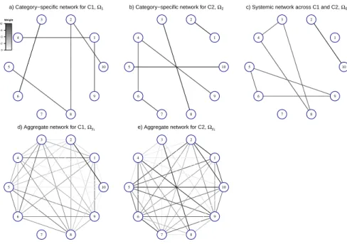
phenomenon is illustrated in Figure 2.1. Category-specific networks Ω

1

and Ω

2

are depicted

for the two categories C1 and C2 (Figure 2.1a,b); these might correspond to, for example,

liver and brain tissue-types.

The systemic network Ω

0

is depicted in Figure 2.1c; this

reflects relationships affecting all tissues at once, for example, gene interactions that are

responsive to hormone levels or other globally-acting processes. Despite the fact that all

three underlying networks, Ω

0

, Ω

1

and Ω

2

, are sparse, the precision matrix of observed

1 2 3 4

5

6

7 8 9

10

a) Category−specific network for C1, Ω1

1 2 3 4

5

6

7 8 9

10

b) Category−specific network for C2, Ω2

1 2 3 4

5

6

7 8 9

10

c) Systemic network across C1 and C2, Ω0

1 2 3 4

5

6

7 8 9

10

d) Aggregate network for C1, Ωy1

1 2 3 4

5

6

7 8 9

10

e) Aggregate network for C2, Ωy2

Weight

0 0.2 0.3 0.4 0.42

Figure 2.1: Illustration of systemic and category-specific networks using a toy example with two

categories (C1 and C2) and p= 10 variables. a) Category-specific network for C1. b)

Category-specific network for C2. c) Systemic network affecting variables in bothC1 and C2. d)Aggregate

network, ΩY1= (Ω−11+ Ω

−1

0 )−1, for categoryC1. e) Aggregate network, ΩY2 = (Ω−21+ Ω

−1

0 )−1, for

C2.

The remainder of the article is organized as follows.

In Section 2.2, we introduce

our dependent Gaussian graphical model, its implementation, and the one-step and EM

methods. In Section 2.3, we study the asymptotic properties of the proposed methods.

In Section 2.4, we illustrate the performance of our methods through simulations and real

mouse study.

2.2

Methodology

For convenience the following notations are used throughout the paper. We denote

the true precision and covariance matrices respectively as Ω

∗

and Σ

∗

. For any matrix

W

= (ω

ij

), we denote the determinant as det(W

), the trace as tr(W

) and

W

−

as the

off-diagonal entries of

W

. We further denote the

jth eigenvalue of

W

as

φ

j

(W

), and the

minimum and maximum eigenvalues of

W

as

φ

min

(W

) and

φ

max

(W

). The Frobenius norm

kW

k

F

is defined as

P

_i,j

ω

_ij2

; the operator/spectral norm

kW

k

2

is defined as

φ

max

(W W

T

);

2.2.1

Problem formulation

In the problem we address, measurements are available on the same

p

outcome variables

in each of

K

distinct categories on each of

n

subjects. Some dependency is anticipated

among outcomes both at the level of the category and at the level of the subject. We

describe dependency at the level of the category as “category-specific”. Drawing an analogy

with physiology, we describe dependency at the level of the subject (i.e., the individual, the

mouse, etc) as “systemic”; that is, modelled as if affecting outcomes in all categories of the

same subject simultaneously. Our primary example is the measurement of gene expression

giving rise to transcript abundance readings on

p

genes on

K

tissues (e.g., liver, kidney,

brain) in

n

laboratory mice. Letting

Yk,i

be the

i-th data vector for the

k-th category, we

model

Y

k,i

=

X

k,i

+

Z

i

(i

= 1, . . . , n;

k

= 1, . . . , K

),

(2.2)

where

Zi

is the random vector corresponding to the shared systemic random effect, and

X

k,i

is the random effect corresponding to the

k-th category. We assume that

X

k,i

and

Zi

are independent and identically distributed

p−dimensional random vectors with mean 0,

and covariance matrices Σk

and Σ

0

respectively, for

i

= 1, . . . , n

and

k

= 1, . . . , K. For

simplicity, we further assume that

Xk,i, and

Zi

are independent of each other and each

follows a multivariate Gaussian distribution.

For the

i-th sample in the

k-th category, we observe the

p-dimensional realization of

Y

k,i

,

vector

y

k,i

= (y

k,i1

, . . . , y

k,ip

)

T

. Without loss of generality, we assume these observations

are centered, i.e.,

P

n

i=1

y

k,ij

= 0 (j

= 1, . . . , p;

k

= 1, . . . , K). Let

y

·,i

be the combined

data vector with

y

·,i

= (y

T_1,i

, . . . , y

_K,iT

)

T

, such that

y

·,i

follows a Gaussian distribution with

covariance ΣY

=

{

_d

Σ

k

}+J

⊗Σ

0

=

{Σ

Y(l,m)

}

1≤l,m≤K

, where

{

d

·}

is a block diagonal matrix,

J

is a square matrix with all 1

0

s as the entries,

⊗

is the Kronecker product and Σ

Y(l,m)

Section 2.6. For simplicity, we write Ω and Σ for

{Ω

_k

}

K

k=0

and

{Σ

k

}

Kk=0

respectively in the

following derivation.

The log-likelihood of the data can be written as

L(Ω

|

y) =

−

npK

2

log(2π) +

n

2

h

log{det(Ω

_Y

)} −

tr( ˆ

Σ

Y

Ω

Y

)

i

,

where

ˆ

ΣY

=

n

−1 n

X

i=1

yiy

_iT

=

{

Σ

ˆ

Y(l,m)

}

1≤l,m≤K

(2.3)

is the

Kp

×

Kp

sample covariance matrix. Under our setting, the log-likelihood can also be

expressed as

L(Ω

|

y)

∝

K

X

k=1

h

log{det(Ω

_k

)} −

tr( ˆ

Σ

_Y(k,k)

Ω

k

)

i

+ log{det(Ω

₀

)}

−

log{det(A)}

+

K

X

l,m=1

tr

Ω

l

Σ

ˆ

Y(l,m)

Ω

m

A

−1

,

(2.4)

where

A

=

P

K

k=0

Ω

k

. The detailed derivation can be found in the Supplementary material.

A natural way to achieve a sparse estimate of Ω is to maximize the penalized

log-likelihood

ˆ

Ω = argmax

Ω0

P(Ω) = argmax

Ω0

L(Ω

|

y)

−

λ

1

K

X

k=1

|Ω

−_k

|

₁

−

λ

2

|Ω

−0

|

1

.

(2.5)

Because the likelihood is complicated in its full form, direct estimation of the precision

matrices in (2.5) is difficult. Estimation can proceed directly, however, given the values

z

of the latent outcome vector

Z. Using this observation and recalling that

Z

∼ N

(0,

Σ

0

),

we can first estimate Σ

0

and then the other parameters subsequently. In Sections 2.2.2 and

2.2.3, we consider estimation of these multiple dependent graphs using a one-step procedure

and a method based on the EM algorithm.

2.2.2

One-step method

cov(Y

l

, Y

m

), for any

m

6=

l, it is natural to use the covariance matrix Σ

Y(l,m)

between all

pairs of

Y

l

and

Ym

to estimate Σ

0

as

ˆ

Σ

0

=

1

K(K

−

1)

X

m6=l

ˆ

Σ

_Y(m,l)

=

1

K(K

−

1)n

X

m6=l n

X

i=1

y

m,i

y

Tl,i

.

(2.6)

Using the fact that var(X

k

) = var(X

k

)

−

var(Z), we can then obtain an estimate for Σ

k

as

ˆ

Σ

k

= ˆ

Σ

Y(k,k)

−

Σ

ˆ

0

=

1

n

n

X

i=1

y

k,i

y

Tk,i

−

Σ

ˆ

0

.

(2.7)

Note that although ˆ

Σk

is symmetric, it is not necessarily positive semidefinite. Positive

definiteness can be ensured, however, using the projection approach of Xu and Shao (2012):

for any possible non-positive definite matrix ˆ

Σ

k

, we obtain the projection ˆ

Σ

0k

by solving

ˆ

Σ

0_k

= argmin

Σ0

kΣ

−

Σk

ˆ

k

∞

.

(2.8)

Lastly, we estimate Ω by minimizing

K

+ 1 separate functions,

W

_k

, defined as follows:

W

_k

(Ω

k

) = tr( ˆ

Σ

0k

Ω

k

)

−

log{det(Ω

k

)}

+

λ

X

i6=j

ω

_k(i,j)

,

(2.9)

where

k

= 0,

1, . . . , K

, and

λ

=

λ

2

when

k

= 0 and

λ

=

λ

1

otherwise. The minimization

problem of (2.9) can be solved efficiently by various algorithms such as GLASSO as proposed

by Friedman et al. (2008) or by QUIC as proposed by Hsieh et al. (2011). We refer to this

approach as the “one-step” method and compare its performance with the EM method

defined next.

2.2.3

Graphical EM method

First, we rewrite the sampling model as



















Z

Y

1

−

Z

..

.

YK

−

Z



















∼ N





































0

0

..

.

0



















,



















Σ

0

0

. . .

0

0

Σ

1

. . .

0

..

.

..

.

..

.

..

.

0

0

. . .

ΣK





































,

and the log-likelihood on the observed data

Y

=

y

as

L(Ω

|

y, z)

∝

log

det(Ω

0

)

−

tr Ω

0

zz

T

/n

+

K

X

k=1

h

log

det(Ω

k

)

−

tr Ω

k n

X

i=1

(y

k,i

−

z

i

)(y

k,i

−

z

i

)

T

/n

i

.

The above log likelihood cannot be calculated directly because the values of

z

i

and

z

i

z

iT

are unobserved. But we can calculate a function

Q(Ω

|

Ω

(t)

, y) in which

z

i

and

z

i

z

iT

are

substituted by their expected values conditional on Ω and

y. This implies the following EM

steps.

E step:

Q(Ω

|

y,

Ω

(t)

)

∝

K

X

k=1

log{det(Ωk)} −

tr

"

ΩkE

(

_n

X

i=1

(yk,i

−

zi)(yk,i

−

zi)

T

/n

|

y,

Ω

(t)

)#!

+ log{det(Ω

0

)} −

tr

(

Ω

0

E

n

X

i=1

ziz

_iT

/n

|

y,

Ω

(t)

!)

=

K

X

k=0

n

log{det(Ω

_k

)} −

tr

Ω

k

Σ

˙

(_kt)

o

.

M step:

Ω

(t+1)

= argmin

Ω

−Q(Ω

|

y,

Ω

(t)

) +

λ

1

X

i6=j K

X

k=1

ω

_k(i,j)

+

λ

₂

X

i6=j

ω

_0(i,j)

,

(2.10)

where Ω

(t)

_and

_ω

(t)

k(i,j)

denote the estimates from the

t-th iteration, and ˙

Σ

(t)

k

is defined as

˙

Σ

(_kt)

=E

(

_n

X

i=1

(y

k,i

−

z

i

)(y

k,i

−

z

i

)

T

/n

|

y,

Ω

(t)

)

= ¨

Σ

Y(k,k)

−

K

X

l=1

¨

Σ

Y(k,l)

Ω

(t)

l

(A

(t)

)

−1

−

(A

(t)

)

−1 K

X

l=1

+ (A

(t)

)

−1 K

X

l,k=1

Ω

(_lt)

Σ

¨

Y(l,k)

Ω

(t)

k

(A

(t)

)

−1

+ (A

(t)

)

−1

,

(k

= 1, . . . , K

).

(2.11a)

˙

Σ

(₀t)

=

n

X

i=1

E z

i

z

Ti

/n

|

y,

Ω

(t)

= (A

(t)

)

−1

+ (A

(t)

)

−1 K

X

l,k=1

Ω

(_lt)

Σ

¨

_Y(l,k)

Ω

(_kt)

(A

(t)

)

−1

,

(2.11b)

where ¨

Σy

is an estimator for Σ

∗_y

, here ¨

Σy

= ˆ

Σy

. Thus, at the

t

+ 1 iteration, problem (2.74)

is decomposed into

K

+ 1 separate optimization problems:

Ω

(_kt+1)

= argmin

Ωk







tr

Ω

k

Σ

˙

(kt)

−

log{det(Ω

_k

)}

+

λ

X

i6=j

ω

_k(i,j)







,

(2.12)

where

λ

=

λ

2

when

k

= 0, otherwise

λ

=

λ

1

for

k

= 0, . . . , K. We then can use GLASSO

(Friedman et al., 2008) to solve (2.12).

We summarize the proposed EM method in the following steps:

Step 1

(Initial value). Initialize ˆ

Σ

0

and ˆ

Σ

k

for all

k

= 1, . . . , K

using (2.3), (2.6), (2.7)

and (2.8).

Step 2

(Updating rule: the M step). Update Ω

k

using (2.12) for all

k

= 0, . . . , K

using

GLASSO.

Step 3

(Updating rule: the E step). Update ˙

Σ

k

using (2.76a) and (2.76a).

Step 4

(Iteration). Iterate Steps 2 and 3 until convergence is achieved.

The next proposition demonstrates the convergence property of our graphical EM

al-gorithm.

Proposition 2.1.

With

λ

1

>

0

and

λ

2

>

0

, the graphical EM algorithm solving

(2.5)

has

the following properties:

1. The penalized log-likelihood in

(2.5)

is bounded above;

2. For each iteration, the penalized log-likelihood is non-decreasing;

3. For a prespecified threshold

δ

, after finite steps, the objective function in

(2.5)

con-verges in the sense that

The detail of proof could be found in the Proof section.

2.2.4

Model selection

We consider two options for selecting the tuning parameter

λ

= (λ

1

, λ

2

), minimization

of the extended BIC (Chen and Chen, 2008), and cross-validation. Extended BIC is quick to

compute and explicitly takes into account both goodness of fit and model complexity.

Cross-validation, by contrast, is more computationally demanding and focuses on the predictive

power of the model.

In our model we define extended BIC as

BIC

γ

(λ) =

−2L({

Ω

ˆ

k

}

Kk=0

) +

ν(λ) log

n

+ 2γ

log

Kp(p

−

1)/2

ν(λ)

,

0

≤

γ

≤

1,

where

{

Ω

ˆ

k

}

Kk=0

are the estimates with the tuning parameter set at

λ,

L(·) is the likelihood

function described in (2.4), the degrees of freedom,

ν

(λ), is the sum of the number of

non-zero off-diagonal elements on

{

Ω

ˆ

k

}

Kk=0

. The criterion is indexed by a parameter

γ

∈

[0,

1].

The tuning parameter

λ

is selected by

ˆ

λ

= argmin{BIC

_γ

(λ) :

λ

1

, λ

2

∈

(0,

∞)}.

In describing the cross-validation procedure, we define the predictive negative

log-likelihood function as follows:

F

(Σ,

Ω) = tr(ΣΩ)

−

log{det(Ω)}.

To select

λ

using cross-validation, we first randomly split the dataset equally into

J

groups, and denote the sample covariance matrix from the

j-th group as Σ

(j,λ)

and the

precision matrix estimated from the remaining groups as ˆ

Ω

(−j,λ)

. Then we choose

λ

as

argmin

λ







J

X

j=1

F(Σ

_(j,λ)

,

Ω

ˆ

(−j,λ)

) :

λ

1

, λ

2

∈

(0,

∞)







.

2.3

Asymptotic properties

In this section we study the asymptotic properties of our proposed methods. First, we

introduce the notation and the regularity conditions on the true precision matrices

{Ω

∗

k

}

Kk=0

,

where Ω

∗_k

= (ω

_k∗_(j,j0₎

)p

×p. Let

T

k

=

n

(j, j

0

) :

j

6=

j

0

, ω

_k∗_(j,j0₎

6= 0

o

be the set of indices of all

nonzero off-diagonal elements in Ω

∗_k

,

q

k

=

|T

k

|

be the cardinality of

T

k

, and

q

=

P

K

k=0

q

k

.

Let

{Σ

∗_k

}

K

k=0

be the true covariance ma

trices for

z

and

{x

_k

}

K

k=1

, and Σ

∗Y

=

{Σ

∗Y(l,m)

}

1≤l,m≤K

be the true covariance matrices for

y. We assume that the following regularity conditions hold.

Condition

1. There exist constants

τ

1

,

τ

2

such that for all

k

= 0,

1, . . . , K, 0

< τ

1

<

φ

min

(Ω

∗k

)

≤

φ

max

(Ω

∗k

)

< τ

2

<

∞.

Condition

2. There exists a constant

τ

3

>

0, such that min

k=0,...,K

min

(j,j0_)∈T

k

ω

∗ k(j,j0₎

≥

τ

3

.

Condition 1 bounds the eigenvalues of Ω

∗_k

, thereby guaranteeing the existence of its

inverse and facilitating the proof of consistency. Condition 2 is needed to bound the nonzero

elements away from zero.

The following theorems discuss estimation consistency and selection sparsistency of our

methods.

Theorem 2.1

(Consistency of the one-step method)

.

Under Conditions 1-2,

(p

+

q) log

p/n

=

o(1)

, and

a

1

(log

p/n)

1/2

≤

λ

1

, λ

2

≤

b

1

{(1 +

p/q) log

p/n}

1/2

for some

con-stants

a

1

and

b

1

. Let

{

Ω

ˆ

k

}

Kk=0

be the minimizer defined by

(2.9)

using the one-step method,

then

K

X

k=0

ˆ

Ω

k

−

Ω

∗k

_F

=

O

p

"

(p

+

q) log

p

n

1/2

#

.

Before we introduce the main theorem of the EM algorithm, we first present a corollary

of Theorem 2.1 which gives a good estimator of Σ

∗_Y

.

Corollary 2.1.

Suppose that Conditions 1-2 hold, and

Ω

ˆ

k

is the one-step solution on

Σ

ˇ

_k

−

Σ

∗_k

F

=

O

p

"

(p

+

q) log

p

n

1/2

#

.

To study our EM estimator, we need a good estimator for Σ

∗_Y

which specifies in the

following condition.

Condition

3. We assume there exists an estimator ˜

Σ

Y

such that

k

ΣY

˜

−

Σ

∗_Y

k

F

=

Op

"

(p

+

q) log

p

n

1/2

#

.

The rate in Condition 3 is required to control the convergence rate of the E-step estimate

˙

Σ

k

and thus the consistency of the estimate from the EM method. Under the conditions in

Theorem 2.1, we can use the one-step estimator ˆ

Ω

0

, . . . ,

ΩK

ˆ

to obtain ˜

ΣY

=

J

⊗

( ˆ

Ω

0

)

−1

+

{

d( ˆ

Ωk)

−1

}, which satisfies Condition 3 by Corollary 2.1.

Theorem 2.2

(Consistency of the EM method)

.

Suppose Conditions 1-3 hold, and

(p

+

q) log

p/n

=

o(1)

, and

a

2

(log

p/n)

1/2

≤

λ

1

, λ

2

≤

b

2

{(1 +

p/q) log

p/n}

1/2

for some constants

a

2

and

b

2

. Then the solution,

{

Ωk

ˆ

}

K_k=0

, of the EM method satisfies

K

X

k=0

Ω

ˆ

k

−

Ω

∗ k

F

=

Op

"

(p

+

q) log

p

n

1/2

#

.

Theorem 2.3

(Sparsistency of the one-step method)

.

Under the assumptions of Theorem

2.1.

If we further assume that

P

K

k=0

Ωk

ˆ

−

Ω

∗ k

=

Op(ηn)

for a sequence of

ηn

→

0

,

and

(log

p/n

+

η

2_n

)

1/2

=

O(λ

1

) =

O(λ

2

)

, then with probability tending to 1, the minimizer

{

Ω

ˆ

k

}

K_k=0

satisfies

ω

ˆ

k(j,j0₎

= 0

for all

(j, j

0

)

∈

T

c

k

,

k

= 0, . . . , K

.

To obtain sparsistency we require a lower bound on the rate of the regularization

pa-rameters

λ

1

and

λ

2

. For consistency, we need an upper bounds for

λ

1

and

λ

2

to control

the biases. In order to have both consistency and sparsistency to hold simultaneously,

we need the bounds to be compatible, that is, we need (log

p/n

+

η

2

n

)

1/2

=

O(λ

1

, λ

2

) =

{(1 +

p/q) log

p/n}

1/2

_{. Using the inequalities}

_kW

_k

2

F

/p

≤ kW

k

2

≤ kW

k

2F

, there are two

scenarios describing the rate of

η

n

, as in Lam and Fan (2009). In the worst case, where

P

K

k=0

k

Ω

ˆ

k

−Ω

∗k

k

has the same rate as

P

K

k=0

k

Ω

ˆ

k

−Ω

∗k

k

F

, the two bounds are compatible only

when

q

=

O(1). In the most optimistic case, where

P

K

k=0

k

Ω

ˆ

k

−Ω

∗k

k

2

=

P

K

Theorem 2.4

(Sparsistency of EM method)

.

Under the assumptions of Theorem 2.2, and

if we further assume that

P

K

k=0

Ω

ˆ

k

−

Ω

∗ k

=

Op(ηn)

and

P

K

k=0

Σ

˜

k

−

Σ

∗ k

=

Op(ζn)

for

sequences of

ηn

→

0

and

ζn

→

0

. Moreover let

ζn

+

ηn

=

O(λ

1

) =

O(λ

2

)

, then with

probability tending to 1, the minimizer

{

Ωk

ˆ

}

K

k=0

in Theorem 2.2 satisfies

ω

ˆ

k(j,j0₎

= 0

for all

(j, j

0

)

∈

T

_kc

,

k

= 0, . . . , K

.

Similar to the discussion above, for the EM algorithm, we have both consistency and

sparsistency when

q

=

O(p) for the best scenario, and

q

=

O(1) for the worst case. Details

of the proof can be found in the Supplementary material.

2.4

Simulation

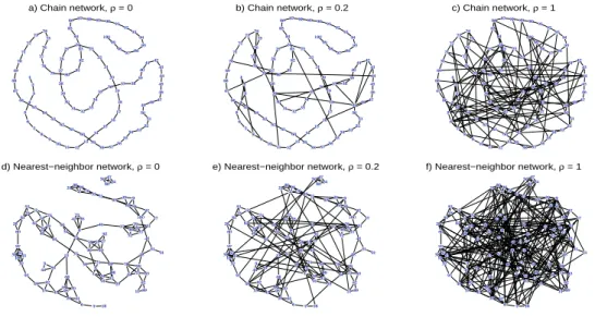
We assessed the performance of the one-step and EM methods by applying them to

simulated data generated by two types of synthetic network: a chain network and a

nearest-neighbor (NN) network (Figure 2.2).

Twenty-four simulation settings were considered.

These varied the base architecture of the category-specific network, the degree to which

the actual structure could deviate from this basic architecture, and the number of outcome

variables (nodes).

● ● ● ● ● ● ● ● ● ● ●● ● ● ● ● ● ● ● ● ● ● ● ● ● ● ● ● ● ● ● ●● ● ● ● ●● ● ● ●● ● ● ● ● ● ● ● ● ● ● ● ● ● ● ● ● ● ● ● ● ● ● ● ● ● ● ● ● ● ● ●● ● ● ● ● ● ●● ● ● ● ● ●●●●● ● ● ● ● ● ● ● ● ● ● 1 2 3 4 5 6 7 8 9 10 1112 13 14 15 16 17 18 19 20 21 22 23 24 25 26 27 28 29 30 31 3233 34 35

36 3738 39 40 4142 43 44 45 46 47 48 49 50 51 52 53 54 55 56 57 58 59 60 61 62 63 64 65 66 67 68 69 70 71 72 7374 75 76 77 78 79 8081

82 83 84 85 868788899091

92 93 94 95 96 97 98 99 100 a) Chain network, ρ = 0

● ● ● ● ● ● ● ● ● ● ●● ● ● ● ● ● ● ● ● ● ● ● ● ● ● ● ● ● ● ● ●● ● ● ● ● ● ● ● ●● ● ● ● ● ● ● ● ● ● ● ● ● ● ● ● ● ● ● ● ● ● ● ● ● ● ● ● ● ● ● ●● ● ● ● ● ● ● ● ● ● ● ● ●●●●● ● ● ● ● ● ● ● ● ● ● 1 2 3 4 5 6 7 8 9 10 1112 13 14 15 16 17 18 19 20 21 22 23 24 25 26 27 28 29 30 31 3233 34 35

36 3738 39 40 4142 43 44 45 46 47 48 49 50 51 52 53 54 55 56 57 58 59 60 61 62 63 64 65 66 67 68 69 70 71 72 7374 75 76 77 78 79 8081

82 83 84 85 868788899091

92 93 94 95 96 97 98 99 100 b) Chain network, ρ = 0.2

● ● ● ● ● ● ● ● ● ● ● ● ● ● ● ● ● ● ● ● ● ● ● ● ● ● ● ● ● ● ● ●● ● ● ● ●● ● ● ●● ● ● ● ● ● ● ● ● ● ● ● ● ● ● ● ● ● ● ● ● ● ● ● ● ● ● ● ● ● ● ●● ● ● ● ● ● ● ● ● ● ● ● ●●●●● ● ● ● ● ● ● ● ● ● ● 1 2 3 4 5 6 7 8 9 10 1112 13 14 15 16 17 18 19 20 21 22 23 24 25 26 27 28 29 30 31 3233 34 35

36 3738 39 40 4142 43 44 45 46 47 48 49 50 51 52 53 54 55 56 57 58 59 60 61 62 63 64 65 66 67 68 69 70 71 72 7374 75 76 77 78 79 8081

82 83 84 85 868788899091

92 93 94 95 96 97 98 99 100 c) Chain network, ρ = 1

● ● ● ● ● ● ● ● ● ● ● ● ● ● ● ● ● ● ● ● ● ● ● ● ● ● ● ● ● ● ● ● ● ● ● ● ● ● ● ● ● ● ● ● ● ● ● ● ● ● ● ● ● ● ● ● ● ● ● ● ● ● ● ● ● ● ● ● ● ● ● ● ● ● ● ● ● ● ● ● ● ● ● ● ● ● ● ● ● ● ● ● ● ● ● ● ● ● ● ● 1 2 3 4 5 6 7 8 9 10 11 12 13 14 15 16 17 18 19 20 21 22 23 24 25 26 27 28 29 30 31 32 33 34 35 36 37 38 39 40 41 42 43 44 45 46 47 48 49 50 51 52 53 54 55 56 57 58 59 60 61 62 63 64 65 66 67 68 69 70 71 72 73 74 75 76 77 78 79 80 81 82 83 84 85 86 87 88 89 90 91 92 93 94 95 96 97 98 99 100 d) Nearest−neighbor network, ρ = 0

● ● ● ● ● ● ● ● ● ● ● ● ● ● ● ● ● ● ● ● ● ● ● ● ● ● ● ● ● ● ● ● ● ● ● ● ● ● ● ● ● ● ● ● ● ● ● ● ● ● ● ● ● ● ● ● ● ● ● ● ● ● ● ● ● ● ● ● ● ● ● ● ● ● ● ● ● ● ● ● ● ● ● ● ● ● ● ● ● ● ● ● ● ● ● ● ● ● ● ● 1 2 3 4 5 6 7 8 9 10 11 12 13 14 15 16 17 18 19 20 21 22 23 24 25 26 27 28 29 30 31 32 33 34 35 36 37 38 39 40 41 42 43 44 45 46 47 48 49 50 51 52 53 54 55 56 57 58 59 60 61 62 63 64 65 66 67 68 69 70 71 72 73 74 75 76 77 78 79 80 81 82 83 84 85 86 87 88 89 90 91 92 93 94 95 96 97 98 99 100 e) Nearest−neighbor network, ρ = 0.2

● ● ● ● ● ● ● ● ● ● ● ● ● ● ● ● ● ● ● ● ● ● ● ● ● ● ● ● ● ● ● ● ● ● ● ● ● ● ● ● ● ● ● ● ● ● ● ● ● ● ● ● ● ● ● ● ● ● ● ● ● ● ● ● ● ● ● ● ● ● ● ● ● ● ● ● ● ● ● ● ● ● ● ● ● ● ● ● ● ● ● ● ● ● ● ● ● ● ● ● 1 2 3 4 5 6 7 8 9 10 11 12 13 14 15 16 17 18 19 20 21 22 23 24 25 26 27 28 29 30 31 32 33 34 35 36 37 38 39 40 41 42 43 44 45 46 47 48 49 50 51 52 53 54 55 56 57 58 59 60 61 62 63 64 65 66 67 68 69 70 71 72 73 74 75 76 77 78 79 80 81 82 83 84 85 86 87 88 89 90 91 92 93 94 95 96 97 98 99 100 f) Nearest−neighbor network, ρ = 1

Figure 2.2: Network topologies generated in the simulations. Top row (a-c) shows chain networks

with noise ratiosρ= 0, 0.2, and 1. Bottom row (d-e) shows nearest-neighbor (NN) networks with