boj12362.pdf

Patterns and drivers of plant functional group

dominance across the Western Hemisphere: a

macroecological re-assessment based on a massive

botanical dataset

KRISTINE ENGEMANN

*, BRODY SANDEL

, BRIAN J. ENQUIST

,

PETER MØLLER JØRGENSEN

_{, NATHAN KRAFT}

_{, AARON MARCUSE-KUBITZA}

_,

BRIAN MCGILL

, NAIA MORUETA-HOLME

, ROBERT K. PEET

, CYRILLE VIOLLE

,

SUSAN WISER

_{and JENS-CHRISTIAN SVENNING}

1_{Section for Ecoinformatics & Biodiversity, Department of Bioscience, Aarhus University, Ny}

Munkegade 114, DK-8000 Aarhus C, Denmark 2

Department of Ecology & Evolutionary Biology, University of Arizona, Biosciences West 310, Tuscon, AZ 85721, USA

3

Missouri Botanical Garden, PO Box 299, St. Louis, MO 63166-0299, USA 4

Department of Biology, University of Maryland, College Park, MD 20742, USA 5

National Center for Ecological Analysis and Synthesis, Santa Barbara, CA 93101-5504, USA 6_{School of Biology and Ecology, University of Maine, Orono, ME 04469, USA}

7_{Integrative Biology, University of California – Berkeley, 3040 VLSB, Berkeley, CA 94720-3140, USA}

8_{Department of Biology CB#3280, University of North Carolina, Chapel Hill, NC 27599-3280, USA}

9_{CEFE UMR 5175, CNRS – Université de Montpellier – Université Paul-Valéry Montpellier – EPHE}

-1919 route de Mende, F-34293 Montpellier, CEDEX 5, France 10_{Landcare Research, PO Box 40, Lincoln 7640, New Zealand}

Received 9 March 2015; revised 9 October 2015; accepted for publication 2 November 2015

Plant functional group dominance has been linked to climate, topography and anthropogenic factors. Here, we assess existing theory linking functional group dominance patterns to their drivers by quantifying the spatial distribution of plant functional groups at a 100-km grid scale. We use a standardized plant species occurrence dataset of unprecedented size covering the entire New World. Functional group distributions were estimated from 3 648 533 standardized occurrence records for a total of 83 854 vascular plant species, extracted from the Botanical Information and Ecology Network (BIEN) database. Seven plant functional groups were considered, describing major differences in structure and function: epiphytes; climbers; ferns; herbs; shrubs; coniferous trees; and angiosperm trees. Two measures of dominance (relative number of occurrences and relative species richness) were analysed against a range of hypothesized predictors. The functional groups showed distinct geographical patterns of dominance across the New World. Temperature seasonality and annual precipitation were most frequently selected, supporting existing hypotheses for the geographical dominance of each functional group. Human influence and topography were secondarily important. Our results support the prediction that future climate change and anthropogenic pressures could shift geographical patterns in dominance of plant functional groups, with probable consequences for ecosystem functioning. © 2015 The Linnean Society of London,Botanical Journal of the Linnean

Society, 2016, 180, 141–160.

ADDITIONAL KEYWORDS: Anthropocene – biodiversity – biogeography – boosted regression trees – climate change – disturbance – macroecology – model averaging – plant functional groups – vegetation modelling.

*Corresponding author. E-mail: [email protected]

Botanical Journal of the Linnean Society, 2016,180, 141–160. With figures

INTRODUCTION

The biosphere can be divided into a number of vegeta-tion zones, thought to be largely determined by climate, that occur in a repeated pattern across the continents (Holdridge, 1947; Küchler, 1949; Olson et al., 2001). The transitions between these zones are believed to be controlled by a variety of primarily climatic factors (Walter, 1973; Whittaker, 1975; Lavorelet al., 1997) that determine the presence and frequency of different functional groups of plants (Dansereau, 1951; Penfound, 1967). However, the extent to which the distributions of these vegetation zones are determined by climate is debated. Other environmental factors related to the availability of resources, or possibly top–down control by grazing or fires, are also believed to influence the distribution of plant vegetation zones (Bond, 2005). The delimitation of such vegetation zones is largely based on dominance patterns among major plant functional groups (Vasquez & Givnish, 1998; Duckworth, Kent & Ramsay, 2000).

We define plant functional groups as species using similar resources and sharing morphological and physiological traits (Lauenroth, Dodd & Sims, 1978; Diaz & Cabido, 1997; Duckworth et al., 2000). The division of plants into functional groupings on the basis of functional traits has been recognized as an important way to simplify ecological complexity and to reveal general patterns (Box, 1996; Cornelissenet al., 2003). Many studies have focused on the connection between functional traits in local communities and environmental factors (Chapin et al., 1996; Bernhardt-Romermann et al., 2011), whereas fewer have looked into continental-scale patterns (e.g. Moles

et al., 2009; Swenson et al., 2012; Lamanna et al.,

2014). Studies that quantitatively investigate continental-scale patterns of plant functional group dominance are lacking. For most species, we have limited knowledge of their individual response to envi-ronmental change and, in turn, how their response might affect the entire community (Bellard et al., 2012). Species in the same functional group are assumed to respond more similarly to changes in their environment, and therefore functional groups can be used as a proxy to investigate the links between species distributions and environmental changes on regional and even global scales (Duckworth et al., 2000; Voigt, Perner & Jones, 2007). Furthermore, plant functional groups based on structure can be easily assigned in the field and are globally comparable among studies and sites (Dormann & Woodin, 2002; Harrisonet al., 2010).

The dominance of different plant functional groups has been linked previously to climate, but the strength and direction of the relationships need

further assessment, especially to improve predictions of climate change effects (Box, 1996; Diaz & Cabido, 1997; Harrison et al., 2010). However, the general importance of geographical variability in other envi-ronmental factors, such as topography, soil conditions and disturbance, is less certain. Humans increasingly change the global environment, exerting a growing pressure on natural ecosystems, and even change natural biomes to anthromes (Ellis, 2011). This is likely to change community composition through dif-ferent effects on difdif-ferent functional groups (Chapin et al., 2000). Which of these multiple factors are the most important for each plant functional group and how they influence geographical patterns of domi-nance are yet to be determined.

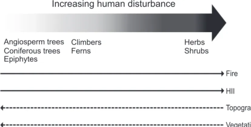
Here, we leverage a massive botanical dataset to provide the first continental-scale quantitative analy-sis of the factors underlying the geographical distribu-tion of major plant funcdistribu-tional groups. We define and compile a new dataset on seven vascular plant func-tional groups that describe important differences in plant structure and function and large-scale vegeta-tion types: ferns and fern allies (hereafter referred to as ferns); coniferous trees; angiosperm trees; shrubs; herbs; climbers; and epiphytes. The aims of this article are: (1) to quantify and compare geographical patterns in the dominance of these plant functional groups across the New World; (2) to identify the underlying environmental drivers; and (3) to determine the rela-tive influence of natural factors compared with human-related disturbance. We assess three hypotheses: (H1) the dominant factors controlling plant functional group distributions are the natural drivers climate and soil; (H2) human influence is now so pervasive that drivers related to anthropogenic disturbance are also important at the continental scale; and (H3) coniferous and angiosperm trees and epiphytes decline in domi-nance with increasing disturbance, whereas herbs and shrubs increase and climbers and ferns exhibit inter-mediate responses (Fig. 1, see also subsection on ‘Specimen data and predictions’ in ‘Material and methods’ section).

MATERIAL AND METHODS

PREDICTOR VARIABLES

We used 12 environmental and biotic predictor vari-ables, all of which have been proposed to be influen-tial for the geographical distribution of plant functional groups (Table 1, Fig. 1). All data layers were resampled to 100 × 100-km2_{resolution grid cells} and projected to the Lambert azimuthal equal area projection. Collinearity among the predictor variables was checked with the pairwise Pearson product-moment correlation coefficient (Supporting

tion, Table S1). We chose annual mean temperature, temperature seasonality, annual precipitation, pre-cipitation seasonality, actual evapotranspiration and the sand content of the soil to represent natural climate- and soil-related factors. The human influence index (HII) and fire were chosen as direct measures of human-related disturbance. HII represents anthropo-genic impacts on the environment as an index value based on nine global data layers related to human population pressure, land use, and infrastructure and accessibility (Wildlife Conservation Society, 2005). Fire was calculated as the mean burnt area per year using data from Tanseyet al. (2008), which provides the Julian date of fire detection each year at 1-km resolution. Tree height also partially captures the effects of human-related disturbance. Tree height con-tains a natural signal reflecting its dependence on climate and other natural environmental factors, but will also strongly reflect anthropogenic land cover change, notably deforestation. In addition, tree height may capture ecological interactions between trees and other functional groups, e.g. negative, competitive interactions with herbs and positive interactions with tree-dependent epiphytes. To avoid issues of circular-ity, tree height was excluded as a predictor of conif-erous and angiosperm trees. We also included elevation, topographical heterogeneity and slope as topographical predictors. Topography will capture natural variation in vegetation structure and distur-bance regime (e.g. landslides in steep terrain). However, it is also likely to contain a human impact signal, as natural vegetation in many regions is increasingly constrained to steep terrain (Sandel & Svenning, 2013). Slope was calculated from elevation as a percentage using the slope tool in the SDMtools

package. Topographical heterogeneity was also calcu-lated from elevation as the standard deviation. Slope and topographical heterogeneity were highly corre-lated (r= 0.97). We chose to retain slope, as this variable is more closely linked to our predictions. Mean annual temperature, temperature seasonality, annual precipitation and actual evapotranspiration were also highly correlated. We defined three sets of models which kept the highly correlated variables separate (Supporting Information, Table S2). Based on improvement in model performance, measured as R2 _{values, of the three model sets, we only report} results from the model with temperature seasonality (model set 2). We also included sampling intensity, calculated as the number of georeferenced observa-tions within a grid cell, as a predictor variable to control further for sampling effects.

SPECIMEN DATA AND PREDICTIONS

We defined seven different vascular plant functional groups, describing important differences in plant structure and function: ferns; coniferous trees; angio-sperm trees; shrubs; herbs; climbers; and epiphytes. Data on plant functional groups were compiled from multiple data sources. We extracted information on plant functional groups from the Botanical Informa-tion and Ecology Network (BIEN 2.0) herbarium col-lection dataset based on the specimen description field (Enquistet al., 2009; http://bien.nceas.ucsb.edu/bien/), the Plant Trait Database (TRY) (Kattge et al., 2011), the SALVIAS database (The SALVIAS Project, 2002; http://www.salvias.net/pages/database_info.php), the USDA PLANTS database (USDA, 2008) and Tropicos® (www.tropicos.org) (Tropicos, 2014). Species were

Herbs

Vegetation HII

Topography Fire Ferns

Climbers

Epiphytes Coniferous trees Angiosperm trees

Increasing human disturbance

Shrubs

Figure 1. Hypothetical relationship between plant functional groups and human disturbance. The large arrow represents a gradient of increasing human disturbance. The positions of the functional groups on the disturbance gradient represent the tolerance of each group based on predictions from the existing literature. The thin arrows show the relationship between human disturbance and our representative environmental predictors: arrows to the right show predictors that increase disturbance, whereas arrows to the left show predictors that decrease disturbance. HII, human influence index.

assigned a functional group value when more than two-thirds of the sources agreed on the same functional group (84 434 species). Otherwise, the species was excluded (5629 species). We then reclassified the species to fit our seven vascular plant functional groups by first dividing the data into three major phylogenetic groups based on their fundamental func-tional differences: ferns; gymnosperms; and angio-sperms. The gymnosperms were subdivided into conifers (mainly trees, although a few are shrubs) and several functionally divergent small groups (e.g. cycads), which were excluded from further considera-tion in this study because of the small sample size. The angiosperms were subdivided into five functional sub-groups: angiosperm trees; shrubs; herbs; climbers; and epiphytes. The shrubs category included both true shrubs and suffruticose species. The climbers were similarly constructed by combining herbaceous vines and woody lianas. Herbs are non-woody herbaceous plants that are not epiphytes or ferns.

Each of our seven functional groups is characterized by unique and ecologically relevant traits. We used this to generate specific predictions about the most influ-ential drivers of the distribution and dominance of each functional group based on the existing literature (see also Table 2).Fernsare vascular cryptogams that disperse via spores (Taylor, Kerp & Hass, 2005). They are also characterized by an independent, free-living gametophyte life stage that is dependent on water (Kato, 1993), and their lack of stomatal control makes them vulnerable to drought (Brodribb & McAdam, 2011). Ferns are limited by water availability, as only a few have adaptations to drought (Schuettpelzet al., 2007). They are therefore expected to peak atsloped

regionsat mid–high elevation and high precipitation

(Aldasoro, Cabezas & Aedo, 2004; Kessleret al., 2011). Epiphytesgrow on other plants, which they rely on only for support, i.e. non-parasitically (Benzing, 1990). They are mostly herbaceous, but also include some woody species (e.g. Clusia L.). The aerial position of epiphytes creates a need for high humidity and hence

high precipitation(Walter, 1973; Benzing, 1990).

Fur-thermore, epiphytes are strongly dependent on avail-able substrate and their distribution is expected to be correlated with the distribution of humid forests. As these forests are often found in mountainous regions, epiphyte richness is expected to peak insloped regions

atintermediate elevation, with drought constriction at

lower elevations, and frost and treeline constriction at higher elevations (Janzen, 1975; Gentry & Dodson, 1987; Kromeret al., 2005).Climbers are defined as herbaceous or woody plants that also non-parasitically rely on other plants for support, but are rooted in the ground. Climbers are more frequent in the tropics because of the vulnerability of their wide vessels to embolisms under freezing conditions (Gentry, 1991). In

T able 1. Names, references and original resolution of environmental predictor variables used in the analyses V ariable Unit Reference Classification T ime span Original resolution Annual mean temperature (Bio 1) °C Hijmans et al ., 2005 Natural 1950–2000 5 ′ T emperature seasonality (Bio 4) Standard deviation × 100 Hijmans et al ., 2005 Natural 1950–2000 5 ′ Annual precipitation (Bio 12) mm Hijmans et al ., 2005 Natural 1950–2000 5 ′ Precipitation seasonality (Bio 15) Coef ficient of variation Hijmans et al ., 2005 Natural 1950–2000 5 ′ Actual evapotranspiration mm/year T rabucco & Zomer , 2010 Natural 1950–2000 30 ′ Elevation m Hijmans et al ., 2005 Natural/anthropogenic 2000 1 k m Slope (derived from elevation) % Hijmans et al ., 2005 Natural/anthropogenic 2000 1 k m T opographical heterogeneity (derived from elevation) Standard deviation Hijmans et al ., 2005 Natural/anthropogenic 2000 1 k m Sand content % Fischer et al ., 2008 Natural 1971–2008 30 ′ Human influence index Index value W ildlife Conservation Society , 2005 Anthropogenic 1995–2004 1 k m Fire (burnt area) Mean T ansey et al ., 2008 Anthropogenic 2000–2007 1 k m T ree height m Lefsky , 2010 Anthropogenic 2003–2007 500 m All datasets were resampled to 100-km resolution. ′ indicates arc seconds.

T able 2. Predictions for plant functional groups Climate T opography Edaphic Disturbance V egetation TSEAS AP PSEAS Elevation Slope Sand HII Fire T reeH. References Ferns L H L M–H M–H W alter , 1973; Janzen, 1975; Gentry & Dodson, 1987; Benzing, 1990; Puigdefábragas & Pugnaire, 1999; Kromer et al ., 2005; Moorhead, Philpott & Bichier , 2010 Epiphytes L H M–H M L H W alter , 1973; Gentry , 1991; Schnitzer , 2005; Jiménez-Castillo, W iser & Lusk, 2007; Cai et al ., 2009 Climbers L L H M H Kato, 1993; Aldasoro et al ., 2004; Bhattarai, V etaas & Grytnes, 2004; Karst, Gilbert & Lechowicz, 2005; Schuettpelz et al ., 2007; W alker & Sharpe, 2010; Brodribb & McAdam, 201 1; Kessler et al ., 201 1 Herbs M–H M H H M–H L Crawley , 1997; V asquez & Givnish, 1998; Gurevitch et al ., 2006; Keddy , 2007; Harrison et al ., 2010 Shrubs M L H H Givnish, 1995; McIntyre et al ., 1999; Puigdefábragas & Pugnaire, 1999; Gurevitch et al ., 2006; Keddy , 2007; Eldridge et al ., 201 1; Zizka et al ., 2014 Coniferous trees M–H L H H L L Bond, 1989; Schulze, Beck, & Müller -Hohenstein, 2002; Gurevitch et al ., 2006; Keddy , 2007 Angiosperm trees L H L M–H L L L Bond, 1989; Crawley , 1997; Puigdefábragas & Pugnaire, 1999; Schulze et al ., 2002; Gurevitch et al ., 2006; Keddy , 2007; Harrison et al ., 2010; Staver et al ., 201 1; T oledo et al ., 201 1; Sandel & Svenning, 2013 Predictions were compiled from the existing literature on functional group dominance along environmental gradients. Dominance along the gradient s was classified as low (L), medium (M), high (H) or unknown (blank). TSEAS, temperature seasonality; AP , annual precipitation; PSEAS, precipitation seas onality; Slope, percentage change in elevation; Sand, percentage of sand in soil; HII, human influence index; Fire, burnt area; T reeH., tree height. For detail so nt h e calculation of the variables, see the ‘Material and methods’ section.

tropical forests, their density increases with drought occurrence as a result of their competitive advantage in the assimilation of carbon and utilization of nitrogen and water compared with trees. Hence, the fraction of climbers should increase withincreasing precipitation

seasonality and decreasing precipitation (Schnitzer,

2005; Cai, Schnitzer & Bongers, 2009). Connected tree crowns support and facilitate climber occurrence by enabling their climbing, and climber distribution should follow the distribution offorests(Toledoet al., 2011), with increases indisturbed areasas a result of strong pioneering abilities (Schnitzer & Bongers, 2011).Herbsgenerally have low water-storing ability and are increasingly found in areas withhigh

precipi-tation (Gurevitch, Scheiner & Fox, 2006). As they

require less carbon for construction, they can occupy colder andmore seasonalenvironments than can trees (Harrison et al., 2010), and competition for light results in higher frequencies of herbs in areas with

open canopiesin unfertile or drought-prone areas with

high soil sand content (Vasquez & Givnish, 1998).

Shrubsare self-standing woody plants that have more than one main stem arising from near the ground, which can prevent fires and herbivores from damaging the innermost stems. Furthermore, the basal meris-tem ensures regrowth in the case of damage to above-ground parts (Zizka, Govender & Higgins, 2014). Shrubs dominate in dry to very dry areas as a result of high drought tolerance (Givnish, 1995), and the shrub fraction should thus increase along an increasing temperature and decreasing precipitation gradient (Gurevitchet al., 2006). The distribution of shrubs can be promoted by disturbance in the form of fires and grazing, which limit the distribution of tree competi-tors and favour the regenerative ability of shrubs (McIntyreet al., 1999; Eldridgeet al., 2011).Treesare self-standing woody plants with a single main stem (Penfound, 1967). We considered two groups of trees: conifers (gymnosperms in the order Pinales); and angiosperm trees. Coniferous trees have mostly evergreen needle-like leaves with deciduous species being rare, whereas angiosperm treesinclude both evergreen and deciduous species, with leaves that are usually broader. The needle-like leaves of conifers have lower photosynthetic ability than the broader leaves of angiosperm trees that dominate productive environ-ments. However, the majority of conifers with ever-green needles have year-round photosynthesis and are more resistant to drought (Bond, 1989). Coniferous trees have low photosynthetic ability of leaves and slow growth, which are competitive disadvantages compared with angiosperm trees in forest openings. This should limit their geographical distribution to colder, more seasonal, drier and nutrient-poor areas

withsandy soils, where angiosperm tree seedlings are

unable to establish (Bond, 1989). Angiosperm trees

require higher amounts of carbon than herbaceous plants for construction, and their frequency should increase with higher water and nutrient availability (Harrison et al., 2010), and dominance should be higher in wetter and less seasonal regions (Crawley, 1997; Toledoet al., 2011).Disturbance in the form of grazing and fires is limiting for the occurrence of both coniferous and angiosperm trees, as it hinders the establishment of seedlings (Bond, 1989; Staver, Archibald & Levin, 2011).

The functional group classification was combined with standardized georeferenced plant species occur-rence data, also from the BIEN 2.0 database. This gave us a total of 83 854 species and 3 648 533 georefer-enced observations with functional group assignments across the New World. The BIEN 2.0 database contains georeferenced plant observations from herbarium specimens, vegetation plot inventories, species distri-bution maps and plant traits covering the whole New World and spanning a wide time period from the beginning of the 17th century to 2011. Most data, however, were from the last few decades. All original data sources can be found on the BIEN website (http:// bien.nceas.ucsb.edu/bien/biendata/bien-2/sources/). Before inclusion in the database, all species names were taxonomically standardized and synonyms updated to the most recent accepted name with the Taxonomic Name Resolution Service (version 1; Boyle et al., 2013), with Tropicos® as the taxonomic author-ity (http://www.tropicos.org) Tropicos, 2014. Also, all specimens in the database were ‘geoscrubbed’ to ensure reliability of georeferenced data. We also excluded all specimens that were categorized as culti-vated to focus on the naturally occurring patterns of plant functional groups.

Two measures of dominance for each functional group were calculated: relative species richness (pro-portion of total plant species richness per 100 × 100-km2 _{grid cell) and relative frequency (proportion of} total number of plant occurrences registered per grid cell). We calculated both measures to ensure that our results were robust. The data were analysed as pro-portions to represent dominance and to reduce any bias affecting the sampling of different functional groups differentially in a given grid cell. We define the dominance of a given functional group as high rela-tive frequency of occurrences or species richness, and refer to it as such in the subsequent sections. The functional group observations were rasterized to 100 × 100-km2 _{grid cells in a Lambert’s azimuthal} equal-area projection to eliminate area effects on species frequency and richness estimates. Total and functional group species richness per grid cell were corrected for differences in sampling intensity between grids using Margalef’s diversity index, before calculating relative richness (Margalef, 1958). This

index standardizes the number of species in a sample in relation to the number of observations following the formulad=S− 1/lnN, whereS is the number of species and N is the number of specimens in the sample (we consider occurrences as specimens and grid cells as samples) (Gamito, 2010). As both of the functional group measures were proportions, they were arcsine transformed before statistical analysis. Sampling intensity varied greatly among cells (range, 1–70 518; median, 48), with poorly sampled cells pos-sibly giving unreliable estimates of growth form domi-nance. Thus, we excluded cells with<50 observations from all statistical analyses, even though this resulted in decreased spatial coverage (Supporting Information, Fig. S1).

STATISTICAL ANALYSIS

We tested the strength of the relationship between the relative richness and relative frequency of each func-tional group and the predictor variables with boosted regression trees (BRTs). The greatest strength of the BRT models is their ability to model non-linear responses and interactions between predictors to opti-mize model fits, whilst overcoming the drawbacks of simple classification and regression trees (CARTs) which have poor predictive performance (De’ath, 2007; Elith, Leathwick & Hastie, 2008). Non-linear responses and interactions are both likely to influence the relationship between functional groups and envi-ronmental predictors, and the BRT models will there-fore provide highly reliable estimates of variable influence. BRTs combine large numbers of CART models adaptively to optimize predictions (Elithet al., 2006; De’ath, 2007). Boosting differs from model aver-aging by being a stagewise procedure. Each CART is fitted randomly, but sequentially, until the addition of new trees no longer increases the accuracy of the model, as measured by model residuals (Greveet al., 2011). We fitted the BRT models to the data using a slow learning rate of 0.001 and allowed for interactions of predictors by setting tree complexity to 5 for increased predictive ability (Leathwick et al., 2008). The influence of interactions between the predictor variables was estimated with the gbm.interactions function in the gbm package. Ten-fold cross-validation was used to determine the optimal number of trees for each functional group, which ranged from 4950 to 11 500 (Table 3, Supporting Information, Table S3), and the bag fraction was set to 0.5 with observations being chosen at random (Elith et al., 2008). The performance of the models was calculated as the cross-validation correlation (Tables 3, S3). We fitted response curves of functional group relative frequency and richness and the environmental variables to

illus-trate the direction of the relationship. Table

3. Percentage contribution of each of the predictor variables for plant functional group species richness dominance TSEAS AP PSEAS Elevation Slope Sand HII Fire T reeH. Sampling No. of trees CV correlation Ferns 12.0 8.5 4.1 5.3 9.9 1 1.8 19.1 7.2 6.1 16.0 10 300 0.68 Epiphytes 26.5 1 1.4 4.6 3.6 5.8 5.3 4.4 6.6 4.4 27.4 7 150 0.80 Climbers 54.0 3.4 2.7 9.8 3.4 2.6 2.2 2.1 2.8 17.1 6 000 0.86 Herbs 75.4 3.5 2.7 2.8 1.4 1.5 2.2 3.4 2.5 4.6 6 100 0.91 Shrubs 16.4 18.1 14.2 8.6 3.4 6.6 6.8 5.8 6.7 13.4 10 200 0.74 Coniferous trees 9.1 5.8 3.7 1.5 8.9 2.3 13.7 13.6 – 41.5 5 350 0.83 Angiosperm trees 58.6 9.7 1.1 5.7 5.6 1.5 7.1 5.0 – 5.5 5 300 0.90 Bold indicates the three most important variables for each functional group in the boosted regression tree (BRT) model. Abbreviations: TSEAS, tempe rature seasonality; AP , annual precipitation; PSEAS, precipitation seasonality; HII, human influence index; T reeH., tree height; Sampling, total number of observations; No. of trees, number of trees fitted; CV correlation, cross-validation correlation.

To supplement the BRT results, we fitted single and multiple ordinary least-squares (OLS) regres-sion models generated with an all subsets selection approach. We used all subsets selection to generate all possible combinations of models from the nine variables in the model set containing temperature seasonality. No pairwise interactions between model parameters were fitted to limit model complexity and to ease the interpretation of parameter coeffi-cients. The model parameters were then calculated as averaged means weighted with the Akaike infor-mation criterion (AIC) of each model, following Burnham & Anderson (2002). Model averaging based on all of these models allowed us to use the models predictively and to compare both the strength and direction of parameter estimates (Symonds & Moussalli, 2010). Model performance was estimated as R2 _{values and model support as} the summed AIC weights across all predictors. Pre-dictor importance was calculated as the summed AIC weight for each individual predictor across all models following the zero method, which substitutes coefficients of predictors not included in the model with zero (Nakagawa & Freckleton, 2010).

Spatial autocorrelation is often present in species occurrence data and can bias parameter estimates (Dormann et al., 2007). We tested for spatial auto-correlation by examining Moran’s I value correlo-grams (Supporting Information, Fig. S2) for the residuals of the OLS model with all the variables for a given predictor variable set. The correlograms showed considerable spatial autocorrelation in all of the global OLS model residuals. Spatial autocorre-lation is only handled to a limited degree by BRT models (Crase, Liedloff & Wintle, 2012), and we therefore repeated all subset selection and model averaging with simultaneous autoregressive (SAR) models, and only show regression results from these. We fitted the SAR models as spatial error models, as these have been shown to account effec-tively for spatial autocorrelation in response and explanatory variables and to provide reliable param-eter estimates (Kissling & Carl, 2008). Similar to the OLS models, no interactions were fitted for the SAR models. Model performance was estimated as pseudo-R2 _{values without the spatial terms, and} model support as the summed AIC weights across all predictors. As a result of computational limits, we only averaged models with ΔAIC<10, as models with higher values have little influence on the final parameter estimates.

All GIS (packages ‘raster’, ‘rgdal’, ‘SDMTools’ and ‘sp’) and statistical (packages ‘ape’, ‘dismo’, ‘fossil’, ‘gbm’, ‘gtools’, ‘Hmisc’, ‘leaps’, ‘MuMIn’, ‘ncf ’, ‘plyr’, ‘qpcR’, ‘spdep’ and ‘vegan’) operations were performed in R 3.0.0 (R Development Core Team, 2013).

RESULTS

SPATIAL PATTERNS OF FUNCTIONAL

GROUP DOMINANCE

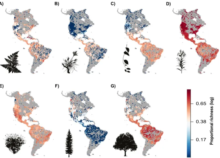
The seven functional groups showed distinct distri-bution patterns in dominance (Fig. 2, r= 0.01–0.83, Supporting Information, Table S4). Epiphytes, climb-ers, ferns and angiosperm trees were most dominant in the tropics, especially in the Amazonian lowland. Herb dominance was highest in the temperate regions and decreased towards tropical regions. Shrub dominance was more patchily distributed, but with reoccurring high dominance in drier regions of both North and South America. Conifers were mainly dominant in North America, with only a few records in South America. The patterns of relative frequency were similar to those of relative richness for all functional groups, and these results are shown in Supporting Information (Figs S3, S4, S5a, S6a; Tables S3–S6).

ENVIRONMENTAL PREDICTORS OF FUNCTIONAL

GROUP DOMINANCE

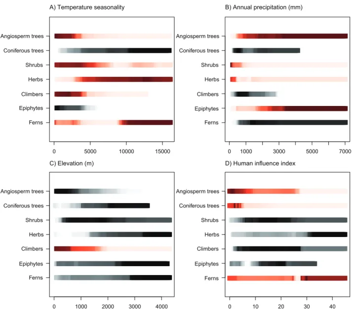
The BRT models showed that temperature seasonal-ity and annual precipitation were most common among the three variables explaining most of the variation in relative dominance for all functional groups, followed by HII and sampling intensity (Table 3). The cross-validation correlation values for the BRT models ranged from 0.68 to 0.91. The fitted response plots from the BRT models showed that epiphytes, climbers, shrubs and angiosperm trees dominated at low temperature seasonality, whereas herbs and conifers peaked at high temperature sea-sonality (Figs 3, S5b). Ferns had maximum domi-nance at high temperature seasonality, but lowest dominance at intermediate temperature seasonality. Epiphytes, ferns and angiosperm trees all had the highest dominance at high annual precipitation, whereas climbers, herbs, shrubs and coniferous trees dominated at low annual precipitation (Figs 3, S5b). Precipitation seasonality was also an important pre-dictor of shrub dominance, with dominance peaking at high seasonality (Fig. S5b). Sand content was only among the more important predictors for ferns and epiphytes, which both peaked at low sand content. Elevation ranked high for climbers, but was generally less important than climatic factors (Table 3). HII was among the most important predictors for ferns and coniferous and angiosperm trees, but was much less important for the other functional groups. Ferns and herbs had highest dominance at medium to high HII, whereas epiphytes, climbers, shrubs and angio-sperm trees peaked at low to intermediate levels of HII. Conifers were only dominant at the lowest levels

of HII (Figs 3, S5b). Sampling ranked high for all functional groups, except shrubs and angiosperm trees (Table 3). Interaction effects were generally weak, but often included a combination of tempera-ture and precipitation variables (Table S6). The only strong interaction was found between sand and HII for ferns, which peaked at low sand content and high HII (Supporting Information, Fig. S7).

Model performance from the SAR multiple regres-sion with all subsets selection was in the range R2_{= 0.25–0.70. The best predictor model for each} functional group consisted of nearly all predictor vari-ables, and so we used model averaging to quantify variable influence. Model averaging showed that tem-perature seasonality was always among the three most important predictors for all functional groups (Table 4). The importance of other predictors varied across the functional groups, but annual precipitation

and sampling were often among the most important predictors. The estimated variable effects were, with few exceptions, consistent with the results from the BRT models (Tables 3, 4).

DISCUSSION

GEOGRAPHICAL PATTERNS IN PLANT FUNCTIONAL

GROUP DOMINANCE

The work of the earliest biogeographers, including Willdenow and von Humboldt, documented changing vegetation patterns along environmental gradients (Lomolino et al., 2010). The differences in geographi-cal patterns of our functional groups (Fig. 2) imply that they are driven by different underlying ecological or evolutionary mechanisms (Wiens, 2011). For instance, having a herbaceous habit has been linked

B) C)

A) D)

E) F) G)

0.17 0.38 0.65

Pr

opor

tional ric

hness (log)

Figure 2. Geographical distribution of relative functional group species richness. All maps show the proportion of individual functional group species richness relative to the total species richness. A, Ferns. B, Epiphytes. C, Climbers. D. Herbs. E, Shrubs. F, Coniferous trees. G, Angiosperm trees. The maps illustrate the unique spatial patterns of relative species richness for the individual functional groups. Richness was calculated as the number of species of a given functional group within a 100 × 100-km2_{grid cell. Cells with<50 observations (Fig. S1C) were excluded. Grey shows cells} without any observations. Projection: Lambert azimuthal equal area.

to cold adaptation (Billings, 1987). Plant functional groups are hypothesized to reflect adaptations to environmental conditions (Box, 1996), which probably explain the differences in their spatial distribution and relation to environmental drivers. Functional groups could also limit the distribution of one another through negative ecological interactions. For example, angiosperm trees are expected to outcompete the more slow-growing coniferous trees under favourable environmental conditions (Bond, 1989). This most probably explains the near-absence of coniferous trees in the Amazonian region of South America where

angiosperm tree dominance peaks (Fig. 2). However, the two functional groups overlap substantially else-where in the Americas, suggesting that the competi-tive dominance of angiosperm trees is also dependent on local conditions. The presence of certain functional groups could also promote the distribution of other functional groups through positive ecological interac-tions. Epiphytes and climbers both rely on woody plants for structural support and substrate, consist-ent with a close distributional overlap with angio-sperm trees. A similar overlap is not found with coniferous trees, as climatic constraints separate

0 5000 10000 15000

A) Temperature seasonality

Epiphytes Climbers

Ferns Herbs Shrubs Coniferous trees Angiosperm trees

0 1000 3000 5000 7000

B) Annual precipitation (mm)

Epiphytes Climbers

Ferns Herbs Shrubs Coniferous trees Angiosperm trees

0 1000 2000 3000 4000

Epiphytes Climbers

Ferns Herbs Shrubs Coniferous trees Angiosperm trees

0 10 20 30 40

Epiphytes Climbers

Ferns Herbs Shrubs Coniferous trees Angiosperm trees

C) Elevation (m) D) Human influence index

Figure 3. Modelled response of plant functional group dominance and environmental predictors obtained from boosted regression tree (BRT) models for the whole New World. The lines represent the relative species richness of a functional group as a function of a given environmental predictor when other predictors in the model are kept constant. Red lines show the three most important predictors for each functional group based on the BRT results (Table 3), whereas black is used for the six least important. The most intense shading shows the environmental conditions at which the functional group reaches highest dominance.

T able 4. Relationship between the distribution of plant functional group species richness and environmental predictors Ferns Epiphytes Climbers Herbs Shrubs Coniferous trees Angiosperm trees Climate TSEAS −0.52 (1) −0.19 (1) − 0.12 (1) 0.93 (1) −0.13 (1) −0.25 (1) −0.78 (1) TSEAS 2 0.48 (1) –– −0.51 (1) −0.05 (0.3) – 0.48 (1) AP 0.01 (0.34) 0.12 (1) −0.08 (1) −0.05 (0.8) −0.49 (1) 0.09 (0.76) 0.26 (1) AP 2 – – −0.00 (0.3) 0.00 (0.3) 0.09 (1) – −0.04 (1) PSEAS −0.03 (0.7) −0.10 (1) 0.04 (1) 0.05 (1) 0.02 (1) 0.03 (0.5) −0.01 (0.6) PSEAS 2 – 0.00 (0.3) 0.05 (1) 0.01 (0.5) – – 0.01 (0.5) T opographic Elevation 0.20 (1) 0.04 (0.6) −0.27 (1) 0.06 (1) −0.00 (0.3) 0.03 (0.48) −0.08 (1) Elevation 2 –– 0.00 (0.3) 0.02 (1) – – −0.02 (0.5) Slope 0.18 (1) 0.06 (0.7) −0.12 (1) −0.01 (0.5) 0.07 (1) 0.01 (0.38) −0.13 (1) Slope 2 – – 0.02 (1) 0.00 (0.2) – – 0.02 (1) Edaphic Sand −0.09 (1) −0.1 1 (1) −0.00 (0.5) −0.00 (0.3) 0.09 (1) 0.02 (0.89) −0.00 (0.4) Sand 2 0.03 (1) – −0.00 (0.2) – – – −0.00 (1) Disturbance HII 0.02 (1) −0.03 (0.5) 0.06 (1) 0.00 (0.3) −0.04 (1) −0.15 (1) −0.01 (1) HII 2 0.01 (0.6) – – – −0.06 (1) 0.00 (0.3) – Fire −0.02 (0.6) −0.08 (0.8) −0.00 (0.4) 0.02 (0.6) −0.06 (1) 0.00 (0.3) 0.00 (0.4) Fire 2 – 0.01 (0.4) 0.00 (0.1) −0.00 (0.2) – – 0.00 (0.14) V egetation related T reeH. 0.13 (1) 0.08 (0.9) 0.08 (1) −0.1 1 (1) −0.07 (1) – – T reeH. 2 – – −0.04 (1) 0.04 (1) 0.05 (1) – – Sampling Samples −0.10 (1) 0.04 (0.7) −0.23 (1) 0.06 (1) −0.3 (1) −0.45 (1) −0.14 (1) Samples 2 0.01 (1) – 0.02 (1) – 0.02 (1) 0.04 (1) 0.01 (1) Model performance R 2 0.26 0.30 0.58 0.70 0.25 0.31 0.60 Functional group richness is relative and proportional to the total number of species. Parameter coef ficients were all standardized and calculated with the simultaneous autoregressive (SAR) model averaging procedure. Numbers in parentheses show the Akaike information criterion (AIC) weight for a give n parameter . Numbers in bold indicate the three most important predictor variables for each growth form (those with the highest coef ficient values). M odel performance was found for the global model. Abbreviations as for T able 3.

these functional groups. Decreasing epiphyte richness at high elevation is linked to treelines, but also to low temperatures, although the physiological mechanism is unknown (Kromer et al., 2005). The geographical pattern found in this study of a near-absence of epi-phytes outside the tropical regions indicates a similar elevational delimitation. Climbers achieve structural support from trees and can invest heavily in their exceptionally efficient vascular system (Schnitzer, 2005). However, this also makes them vulnerable to freezing-induced embolisms (Gallagher & Leishman, 2012) and explains the low climber dominance in the colder areas inhabited by conifers.

CLIMATIC AND NON-CLIMATIC NATURAL DRIVERS OF

GEOGRAPHICAL PATTERNS

The importance of climatic factors for all functional groups (Table 3) supports hypothesis H1 and shows the strong influence of climate on plant communities through water availability (Walter, 1973), consistent with interactions between climatic predictors (Table S6). Our results were generally consistent with predictions from the literature (Table 2) and quanti-tatively confirm the strong link between plant func-tional groups and climate. The climatic predictors explained 24.6–81.6% of all explained variance (sum of percentage contribution, Table 3), emphasizing the high importance of climate for large-scale geographi-cal patterns of plant functional groups.

Trees require larger amounts of carbon for construc-tion than do smaller plants and are expected to domi-nate in warmer and wetter environments, with the opposite being true for smaller plants, such as shrubs and herbs (Harrisonet al., 2010). Angiosperm trees are dominant in the most favourable environments, whereas herbs are dominant in areas with higher temperature seasonality and lower precipitation, and shrubs are clearly dominant in the driest areas where high precipitation seasonality increases the risk of drought events. Conifers are dominant in cold and dry areas environmentally opposite to angiosperm trees, consistent with our predictions (Table 2), but are not strongly linked to any climatic predictor. We also found the predicted division in climatic preference for epi-phytes and climbers (Table 2). Both have their highest relative dominance under tropical conditions. However, the epiphytes, which require high humidity (Benzing, 1990), are dominant in wetter areas, whereas climbers are dominant in drier areas, consist-ent with their strong ability to extract and contain water (Schnitzer, 2005). Ferns are dominant in areas of high annual precipitation (Fig. 3), reflecting high water dependence and a preference for mesic habitats (Kato, 1993). A study from Africa, however, has shown that fern species richness is underestimated for arid

regions (Anthelme, Abdoulkader & Viane, 2011). This pattern might be similar for the New World if sampling of ferns was focused on humid areas. Insufficient sampling could explain why the fern models showed low performance.

Previous climate change events have resulted in shifting communities and changing functional compo-sition (Davis & Shaw, 2001; Cárdenas et al., 2014). The strong connection to climate suggests that current and future climate change can severely influ-ence spatial patterns of plant functional group domi-nance. Encroachment of woody shrubs and trees into grasslands has been documented for North American grasslands (Knapp et al., 2008) and increases in climbers have been found for tropical forests (Schnitzer & Bongers, 2011), whereas epiphytes and trees have been identified as especially prone to extinction risk (Leãoet al., 2014). This illustrates that plant functional group responses to climate change are complex and worthy of further investigation.

The topographic predictors elevation and slope are also strong predictors of some functional groups (Table 3), consistent with local-scale studies (e.g. Waide et al., 1999; Moeslund et al., 2013). Both are positively related to both epiphyte and fern relative richness, confirming the prediction of high dominance of both functional groups in humid montane rainfor-ests (Figs 3, S5b; Table 2) (Benzing, 1990). Global forest cover is strongly correlated with increasing slope as a result of anthropogenic land clearing on more accessible low slope areas (Sandel & Svenning, 2013). We also found a positive relationship between slope and both shrubs and coniferous trees, whereas the relationship was negative for angiosperm trees (Figs 3, S5b; Table 2). The generally slower growing conifers only have a competitive advantage over angiosperm trees in cold or nutrient-poor areas (Bond, 1989), consistent with a strong connection to temperature seasonality (Table 3) and clear conifer dominance in the coldest and highest areas (Figs 3, S5b).

Tree height was included as a proxy for ecological interactions between trees and other functional groups. Epiphytes and climbers dominate at increas-ing tree height (Fig. S5b), consistent with the need of both groups for trees for support (Benzing, 1990). Tree height generally ranks low for the functional groups. Our spatial resolution may be too coarse to determine the importance of species interactions, which more probably influence local-scale patterns (McGill, 2010). Alternatively, tree height may not be representative of interactions affecting functional group distribution, despite canopy density having strong local effects (Oberle, Grace & Chase, 2009). We also expected a strong link to soil conditions, but only found a strong effect for ferns, showing that other environmental factors are more important at this bicontinental scale.

HUMAN INFLUENCE

Humans have transformed natural ecosystems world-wide, and future land use changes are likely to esca-late anthropogenic impacts (Ellis, 2011). HII is strongly related to ferns with dominance at medium to high HII (Fig. 3). A positive connection to HII could be a result of higher sampling in areas closer to cities and infrastructure (Reddy & Da, 2003). Whether this effect influences ferns more than other functional groups is uncertain, but should be explored further. Increased sampling focused on ferns might also improve model explanatory power, which is particu-larly low for this functional group (Table 3). On the contrary, there is no indication that ferns are particu-larly poorly sampled. The connection to HII could simply be caused by ferns and humans occupying similar conditions, consistent with a strong interac-tion between sand and HII (Fig. S7). Many ferns are rapid colonizers and thus tolerant of disturbance, with many being clearly well adapted and even ben-efitting from disturbance (Arens & Baracaldo, 1998; Jenkins & Parker, 2000; Slocumet al., 2004). Global forest cover has been negatively affected by land clearing (Hansenet al., 2013) and is a probable cause of the strong and negative relationship between HII and coniferous and angiosperm trees. This result highlights the fact that natural forest ecosystems have been and still are pressurized by human land use changes (Butchartet al., 2010). Other functional groups might benefit from human-mediated dispersal, disturbance or land use changes (Ellis, Antill & Kreft, 2012). For instance, shrubs are, in some cases, pro-moted by grazing (Roques, O’Connor & Watkinson, 2001), although the functional group is not strongly correlated with HII (Table 3). Grazing is difficult to measure at large scales and is unlikely to be captured well by HII, explaining the weak connection to shrub dominance.

Whether plant distributions are controlled by resources (e.g. light or water) or consumers (grazers or fire) has been much debated (Hairston, Smith & Slobodkin, 1960; Bond, 2005). We expected fire to affect shrub dominance strongly, as this functional group has been known to be promoted by fires (Knapp

et al., 2008; Papanikolaou et al., 2011). However, the

effect is rather weak (Table 3). Conifers are strongly and negatively affected by fire, consistent with defor-estation after fires (Bond, 1989). Fires strongly affect local plant communities, but the effect is weak com-pared with the other environmental predictors at our continental scale. This pattern is consistent with results from a previous study covering the African continent (Greve et al., 2011). High-impact fires are, however, expected to increase in frequency and sever-ity with future climate change to the extent of

gradu-ally shifting vegetation zones at larger scales (Bowmanet al., 2011; Staver et al., 2011).

Overall, these results show that natural environ-mental predictors are not the only influential drivers of functional group dominance at the continental scale. Human activities also shape large-scale biogeo-graphical patterns, supporting hypothesis H2. The responses to disturbance are mostly consistent with hypothesis H3, showing that disturbance and human activities can affect broad-scale vegetation patterns via interactions with plant functional traits.

METHODOLOGICAL CONSIDERATIONS

Increased sampling near roads, cities and rivers can create strong spatial sampling bias (Schulman, Toivonen & Ruokolainen, 2007) and can severely affect species richness estimates (Gotelli & Colwell, 2001; Engemann et al., 2015). Despite the use of the Margalef correction and inclusion of sampling inten-sity in our models, the positive correlation to HII by epiphytes and ferns might be caused by sampling bias, although neither was the least sampled func-tional group (Supporting Information, Fig. S8). Conif-erous trees were the least sampled functional group in our dataset and also had the strongest correlation to sampling (Table 4). Most functional groups only varied slightly with sampling intensity, whereas herbs and angiosperm trees showed more variation (Supporting Information, Fig. S9), and it is possible that the functional groups are differently sampled. The effect of spatial sampling bias could be further explored by investigating distances to roads, cities and herbaria for each functional group. The strong effect of sampling emphasizes the underlying issue of sampling bias in unstandardized datasets compiled from multiple sources (Martin, Blossey & Ellis, 2012; Amano & Sutherland, 2013). A promising new approach is stacking of species distribution models (Dubuis et al., 2011) which are less affected by sam-pling (Loiselle et al., 2008). Such maps are increas-ingly being made available from diversity databases (e.g. BIEN 2013, http://bien.nceas.ucsb.edu/bien/; Map of Life, www.mappinglife.org).

Spatial autocorrelation can influence the impor-tance of parameter estimates (Kissling & Carl, 2008). We used SAR as a supplement to BRT models, as these do not entirely account for spatial dependence in model residuals. The predictive ability of BRT models and validity of cross-validation values could be improved by specifically handling spatial relation. Although sampling bias and spatial autocor-relation could influence our results (Kissling & Carl, 2008; Michalcová et al., 2011), both modelling approaches concurred on the most important drivers of functional group dominance (Tables 3, 4).

FUTURE PERSPECTIVES

The definition of plant functional types is an impor-tant aspect of dynamic modelling of vegetation responses (DGVMs) to climate change (Harrison et al., 2010). We have quantitatively shown that plant functional group dominance shifts along natural cli-matic gradients across two continents. The use of functional groups ensures that our results are glob-ally comparable (Duckworthet al., 2000). The congru-ence between our results and predicted relationships shows that our dataset and analytical approach are robust. The results can be used complementarily to the functional types employed in DGVMs (see, for example, Scheiter & Higgins, 2009). In addition, we also showed that these large-scale patterns are influ-enced by anthropogenic disturbance. Synergistic effects of multiple pressures could cause greater effects than observed for each predictor alone (Brook, Sodhi & Bradshaw, 2008), and should be included in dynamic models aimed at predicting vegetation response. Different drivers work at different scales (McGill, 2010) and future work should focus on testing predictor scale dependence for functional groups. However, we found that strong sampling effects and increasing resolution to a finer grain would increase the effect of sampling bias as spatial coverage decreases.

All functional groups showed clear and strong con-nections to climate previously not confirmed statisti-cally for a dataset covering the whole New World. Natural environmental predictors were not the only influential drivers of functional group dominance. Disturbance and human activities also affected domi-nance of the functional groups through functional responses. Future climate change in combination with increased anthropogenic pressures has the potential to shift the geographical distribution of functional vegetation groups and to affect ecosystem function through changes in plant community func-tional composition.

ACKNOWLEDGEMENTS

This work was conducted as part of the Botanical Information and Ecology Network (BIEN) Working Group (PIs B.J.E., Richard Condit, R.K.P., Brad Boyle, Steven Dolins and Barbara M. Thiers) sup-ported by the National Center for Ecological Analysis and Synthesis, a center funded by the National Science Foundation (Grant #EF-0553768), the Uni-versity of California, Santa Barbara, and the State of California. The BIEN Working Group was also sup-ported by the iPlant collaborative (National Science Foundation #DBI-0735191; URL: www.iplantcollabo-rative.org). We thank all the contributors (see http://

bien.nceas.ucsb.edu/bien/people/data-providers/ for a full list) for the invaluable data provided to BIEN. We also thank Z. Wang, A. Barfod, R. Field, J. Bailey and an anonymous referee for comments on earlier ver-sions of this paper. Funding for K.E. was provided through Aarhus University. J.-C.S. was supported by the European Research Council (ERC-2012-StG-310886-HISTFUNC). NM-H acknowledges support by an Elite-Forsk Award and the Aarhus University Research Foundation.

REFERENCES

Aldasoro JJ, Cabezas F, Aedo C. 2004. Diversity and distribution of ferns in sub-Saharan Africa, Madagascar and

some islands of the South Atlantic.Journal of Biogeography

31:1579–1604.

Amano T, Sutherland WJ. 2013.Four barriers to the global understanding of biodiversity conservation: wealth,

lan-guage, geographical location and security.Proceedings of the

Royal Society of London B: Biological Sciences 280:

20122649.

Anthelme F, Abdoulkader A, Viane R. 2011.Are ferns in arid environments underestimated? Contribution from the

Saharan Mountains.Journal of Arid Environments75:516–

523.

Arens NC, Baracaldo PS. 1998.Distribution of tree ferns (Cyatheaceae) across the successional mosaic in an Andean

cloud forest, Narino, Colombia.American Fern Journal88:

60–71.

Bellard C, Bertelsmeier C, Leadley P, Thuiller W, Courchamp F. 2012. Impacts of climate change on the

future of biodiversity.Ecology Letters15:365–377.

Benzing DH. 1990. Vascular epiphytes. Cambridge: Cam-bridge University Press.

Bernhardt-Romermann M, Gray A, Vanbergen AJ, Berges L, Bohner A, Brooker RW, De Bruyn L, De Cinti B, Dirnbock T, Grandin U, Hester AJ, Kanka R, Klotz S, Loucougaray G, Lundin L, Matteucci G, Meszaros I, Olah V, Preda E, Prevosto B, Pykala J, Schmidt W, Taylor ME, Vadineanu A, Waldman T. 2011.Functional traits and local environment predict veg-etation responses to disturbance: a pan-European multi-site

experiment.Journal of Ecology99:777–787.

Bhattarai KR, Vetaas OR, Grytnes JA. 2004.Fern species richness along a central Himalayan elevational gradient,

Nepal.Journal of Biogeography31:389–400.

Billings WD. 1987.Constraints to plant growth,

reproduc-tion, and establishment in arctic environments.Arctic and

Alpine Research19:357–365.

Bond WJ. 1989.The tortoise and the hare: ecology of

angio-sperm dominance and gymnoangio-sperm persistence.Biological

Journal of the Linnean Society36:227–249.

Bond WJ. 2005.Large parts of the world are brown or black:

a different view on the ‘Green World’ hypothesis.Journal of

Vegetation Science16:261–266.

Bowman DMJS, Balch J, Artaxo P, Bond WJ, Cochrane MA, D’Antonio CM, Defries R, Johnston FH, Keeley

JE, Krawchuk MA, Kull CA, Mack M, Moritz MA, Pyne S, Roos CI, Scott AC, Sodhi NS, Swetnam TW, Whittaker R. 2011.The human dimension of fire regimes

on Earth.Journal of Biogeography38:2223–2236.

Box EO. 1996. Plant functional types and climate at the

global scale.Journal of Vegetation Science7:309–320.

Boyle B, Hopkins N, Lu Z, Raygoza Garay JA, Mozzherin D, Rees T, Matasci N, Narro ML, Piel WH, McKay SJ, Lowry S, Freeland C, Peet RK, Enquist BJ. 2013.The taxonomic name resolution service: an online tool

for automated standardization of plant names.BMC

Bioin-formatics14:16.

Brodribb TJ, McAdam SAM. 2011. Passive origins of

sto-matal control in vascular plants.Science331:582–585.

Brook BW, Sodhi NS, Bradshaw CJA. 2008. Synergies

among extinction drivers under global change. Trends in

Ecology & Evolution23:453–460.

Burnham KP, Anderson DR. 2002. Model selection and inference: a practical information theoretic approach,Second edition. New York: Springer-Verlag.

Butchart SSHM, Walpole M, Collen B, Van Strien A, Scharlemann JPW, Almond REA, Baillie JEM, Bomhard B, Brown C, Bruno J, Carpenter KE, Carr GM, Chanson J, Chenery AM, Csirke J, Davidson NC, Dentener F, Foster M, Galli A, Galloway JN, Genovesi P, Gregory RD, Hockings M, Kapos V, Lamarque J-F, Leverington F, Loh J, McGeoch MA, McRae L, Minasyan A, Hernández Morcillo M, Oldfield TEE, Pauly D, Quader S, Revenga C, Sauer JR, Skolnik B, Spear D, Stanwell-Smith D, Stuart SN, Symes A, Tierney M, Tyrrell TD, Vié J-C, Watson R. 2010.Global

biodiversity: indicators of recent declines. Science 328:

1164–1168.

Cai ZQ, Schnitzer SA, Bongers F. 2009.Seasonal differ-ences in leaf-level physiology give lianas a competitive

advantage over trees in a tropical seasonal forest.Oecologia

161:25–33.

Cárdenas ML, Gosling WD, Pennington RT, Poole I, Sherlock SC, Mothes P. 2014. Forests of the tropical

eastern Andean flank during the middle Pleistocene.

Pal-aeogeography, Palaeoclimatology, Palaeoecology393:76–89. XChapin FS, Bret-Harte MS, Hobbie SE, Zhong H. 1996.

Plant functional types as predictors of transient responses

of arctic vegetation to global change.Journal of Vegetation

Science7:347–358.

Chapin FS, Zavaleta ES, Eviner VT, Naylor RL, Vitousek PM, Reynolds HL, Hooper DU, Lavorel S, Sala OE, Hobbie SE, Mack MC, Díaz S. 2000.

Conse-quences of changing biodiversity.Nature405:234–242.

Cornelissen JHC, Lavorel S, Garnier E, Díaz S, Buchmann N, Gurvich DE, Reich PB, ter Steege H, Morgan HD, Van Der Heijden MG A, Pausas JG, Poorter H. 2003.A handbook of protocols for standardised and easy measurement of plant functional traits worldwide. Australian Journal of Botany51:335–380.

Crase B, Liedloff AC, Wintle BA. 2012.A new method for dealing with residual spatial autocorrelation in species

dis-tribution models.Ecography35:879–888.

Crawley MJ. 1997.The structure of plant communities. Plant ecology. Malden: Blackwell Science Ltd, 475–532.

Dansereau P. 1951.Description and recording of vegetation

upon a structural basis.Ecology32:172–229.

Davis MB, Shaw RG. 2001. Range shifts and adaptive

responses to Quaternary climate change.Science292:673–

679.

De’ath G. 2007. Boosted trees for ecological modeling and

prediction.Ecology 88:243–251.

Diaz S, Cabido M. 1997.Plant functional types and

ecosys-tem function in relation to global change. Journal of

Veg-etation Science8:463–474.

Dormann CF, McPherson JM, Araújo MB, Bivand R, Bolliger J, Carl G, Davies RG, Hirzel A, Jetz W, Kissling DW, Kühn I, Ohlemüller R, Peres-Neto PR, Reineking B, Schröder B, Schurr FM, Wilson R. 2007.

Methods to account for spatial autocorrelation in the

analy-sis of species distributional data: a review. Ecography30:

609–628.

Dormann CF, Woodin SJ. 2002. Climate change in the Arctic: using plant functional types in a meta-analysis of

field experiments.Functional Ecology16:4–17.

Dubuis A, Pottier J, Rion V, Pellissier L, Theurillat JP, Guisan A. 2011.Predicting spatial patterns of plant species richness: a comparison of direct macroecological and species

stacking modelling approaches.Diversity and Distributions

17:1122–1131.

Duckworth JC, Kent M, Ramsay PM. 2000. Plant func-tional types: an alternative to taxonomic plant community

description in biogeography? Progress in Physical

Geogra-phy24:515–542.

Eldridge DJ, Bowker MA, Maestre FT, Roger E, Reynolds JF, Whitford WG. 2011. Impacts of shrub encroachment on ecosystem structure and functioning:

towards a global synthesis.Ecology Letters14:709–722.

Elith J, Graham CH, Anderson RP, Dudík M, Ferrier S, Guisan A, Hijmans RJ, Huettmann F, Leathwick JR, Lehmann A, Li J, Lohmann LG, Loiselle BA, Manion G, Moritz C, Nakamura M, Nakazawa Y, Overton JMcC, Townsend Peterson A, Phillips SJ, Richardson K, Scachetti-Pereira R, Schapire RE, Soberón J, Williams S, Wisz MS, Zimmermann NE. 2006. Novel methods improve prediction of species’ distributions from

occurrence data.Ecography29:129–151.

Elith J, Leathwick JR, Hastie T. 2008.A working guide to

boosted regression trees. Journal of Animal Ecology 77:

802–813.

Ellis EC. 2011. Anthropogenic transformation of the

terres-trial biosphere.Philosophical Transactions. Series A,

Math-ematical, Physical, and Engineering Sciences 369: 1010– 1035.

Ellis EC, Antill EC, Kreft H. 2012. All is not loss: plant

biodiversity in the Anthropocene.PLoS ONE7:e30535.

Engemann K, Enquist BJ, Sandel B, Boyle B, Jørgensen PM, Morueta-Holme N, Peet RK, Violle C, Svenning JC. 2015. Limited sampling hampers ‘big data’ estimation

of species richness in a tropical biodiversity hotspot.Ecology

and Evolution5:807–820.

Enquist BJ, Condit R, Peet B, Schildhauer M, Thiers B, The BIEN working group. 2009.The Botanical and Infor-mation Ecology Network (BIEN): cyberinfrastructure for an integrated botanical information network to investigate the ecological impacts of global climate change on plant biodi-versity. Available at http://www.iplantcollaborative.org/sites/ default/files/BIEN_White_Paper.pdf

Fischer G, Nachtergaele F, Prieler S, van Velthuizen S, Verelst L, Wiberg D. 2008. Global Agro-ecological Zones Assessment for Agriculture (GAEZ 2008). IIASA, Laxenburg, Austria and FAO, Rome, Italy. Available at: http://www .fao.org/soils-portal/soil-survey/soil-maps-and-databases/

harmonized-world-soil-database-v12/en/ (accessed 10

October 2008).

Gallagher RV, Leishman MR. 2012. A global analysis of trait variation and evolution in climbing plants (P Ladiges,

Ed.).Journal of Biogeography39:1757–1771.

Gamito S. 2010.Caution is needed when applying Margalef

diversity index.Ecological Indicators10:550–551.

Gentry AH. 1991.The distribution and evolution of climbing

plants. In: Putz FE, Mooney HA, eds. Biology of vines.

Cambridge: Cambridge University Press, 3–49.

Gentry AH, Dodson CH. 1987.Diversity and biogeography

of Neotropical vascular epiphytes. Annals of the Missouri

Botanical Garden74:205–233.

Givnish TJ. 1995.Plant stems: biomechanical adaptation for energy capture and influence on species distributions. In:

Gartner BL, ed. Plant stems: physiology and functional

morphology. San Diego, CA: Academic Press, 3–49.

Gotelli NJ, Colwell RK. 2001. Quantifying biodiversity: procedures and pitfalls in the measurement and comparison

of species richness.Ecology Letters4:379–391.

Greve M, Lykke AM, Blach-Overgaard A, Svenning JC. 2011. Environmental and anthropogenic determinants of

vegetation distribution across Africa. Global Ecology and

Biogeography20:661–674.

Gurevitch J, Scheiner SM, Fox GA. 2006. The ecology of plants. Sunderland: Sinauer Associates.

Hairston NG, Smith FE, Slobodkin LB. 1960.Community

structure, population control, and competition. American

Naturalist94:421–425.

Hansen MC, Potapov PV, Moore R, Hancher M, Turubanova SA, Tyukavina A, Thau D, Stehman SV, Goetz SJ, Loveland TR, Kommareddy A. 2013. High-resolution global maps of 21st-century forest cover change. Science342:850–853.

Harrison SP, Prentice IC, Barboni D, Kohfeld KE, Ni J, Sutra JP. 2010. Ecophysiological and bioclimatic

founda-tions for a global plant functional classification.Journal of

Vegetation Science21:300–317.

Hijmans RJ, Cameron SE, Parra JL, Jones PG, Jarvis A. 2005.Very high resolution interpolated climate surfaces for

global land areas.International Journal of Climatology25:

1965–1978.

Holdridge LR. 1947. Determination of World plant

forma-tions from simple climatic data.Science105:367–368.

Janzen D. 1975. Ecology of plants in the tropics. London: Edward Arnold.

Jenkins MA, Parker GR. 2000.The response of herbaceous-layer vegetation to anthropogenic disturbance in intermit-tent stream bottomland forests of southern Indiana, USA. Plant Ecology151:223–237.

Jiménez-Castillo M, Wiser SK, Lusk CH. 2007.Elevational parallels of latitudinal variation in the proportion of lianas

in woody floras.Journal of Biogeography34:163–168.

Karst J, Gilbert B, Lechowicz MJ. 2005.Fern community assembly: the roles of chance and the environment at local

and intermediate scales.Ecology86:2473–2486.

Kato M. 1993. Biogeography of ferns: dispersal and

vicari-ance.Journal of Biogeography20:265–274.

Kattge J, Díaz S, Lavorel S, Prentice IC, Leadley P, Bönisch G, Garnier E, Westoby M, Reich PB, Wright IJ, Cornelissen JHC, Violle C, Harrison SP, Van Bodegom PM, Reichstein M, Enquist BJ, Soudzilovskaia NA, Ackerly DD, Anand M, Atkin O, Bahn M, Baker TR, Baldocchi D, Bekker R, Blanco CC, Blonder B, Bond WJ, Bradstock R, Bunker DE, Casanoves F, Cavender-Bares J, Chambers JQ, Chapin FS, Chave J, Coomes D, Cornwell WK, Craine JM, Dobrin BH, Duarte L, Durka W, Elser J, Esser G, Estiarte M, Fagan WF, Fang J, Fernández-Méndez F, Fidelis A, Finegan B, Flores O, Ford H, Frank D, Freschet GT, Fyllas NM, Gallagher RV, Green WA, Gutierrez AG, Hickler T, Higgins S, Hodgson JG, Jalili A, Jansen S, Joly C, Kerkhoff AJ, Kirkup D, Kitajima K, Kleyer M, Klotz S, Knops JMH, Kramer K, Kühn I, Kurokawa H, Laughlin D, Lee TD, Leishman M, Lens F, Lenz T, Lewis SL, Lloyd J, Llusià J, Louault F, Ma S, Mahecha MD, Manning P, Massad T, Medlyn B, Messier J, Moles AT, Müller SC, Nadrowski K, Naeem S, Niinemets Ü, Nöllert S, Nüske A, Ogaya R, Oleksyn J, Onipchenko VG, Onoda Y, Ordoñez J, Overbeck G, Ozinga WA, Patiño S, Paula S, Pausas JG, Peñuelas J, Phillips OL, Pillar V, Poorter H, Poorter L, Poschlod P, Prinzing A, Proulx R, Rammig A, Reinsch S, Reu B, Sack L, Salgado-Negret B, Sardans J, Shiodera S, Shipley B, Siefert A, Sosinski E, Soussana J-F, Swaine E, Swenson N, Thompson K, Thornton P, Waldram M, Weiher E, White M, White S, Wright SJ, Yguel B, Zaehle S, Zanne AE, Wirth C. 2011.

TRY – a global database of plant traits. Global Change

Biology17:2905–2935.

Keddy PA. 2007. Plants and vegetation. Cambridge: Cam-bridge University Press.

Kessler M, Kluge J, Hemp A, Ohlemüller R. 2011.A global comparative analysis of elevational species richness patterns

of ferns.Global Ecology and Biogeography20:868–880.

Kissling WD, Carl G. 2008.Spatial autocorrelation and the

selection of simultaneous autoregressive models. Global

Ecology and Biogeography17:59–71.

Knapp AK, Briggs JM, Collins SL, Archer SR, Bret-Harte MS, Ewers BE, Peters DP, Young DR, Shaver GR, Pendall E, Cleary MB. 2008. Shrub encroachment in North American grasslands: shifts in growth form dominance rapidly alter control of ecosystem

carbon inputs.Global Change Biology14:615–623.