Tang_unc_0153D_14708.pdf

(1)

ASSOCIATION ANALYSIS OF RARE VARIANTS IN SEQUENCING STUDIES

Zhengzheng Tang

A dissertation submitted to the faculty of the University of North Carolina at Chapel Hill in partial fulfillment of the requirements for the degree of Doctor of Philosophy in

the Department of Biostatistics in the Gillings School of Global Public Health.

Chapel Hill 2014

Approved by:

Dr. Danyu Lin

Dr. Donglin Zeng

Dr. Wei Sun

Dr. Yun Li

(2)

(3)

ABSTRACT

ZHENGZHENG TANG: Association Analysis of Rare Variants in Sequencing Studies

(Under the direction of Dr. Danyu Lin)

Recent advances in sequencing technologies have made it possible to explore the

influence of rare variants on complex diseases and traits. Large-scale sequencing studies

provide the opportunity to examine the proportion of the missing heritability that is

attributable to rare variants. They also pose a range of analytical and computational

challenges that cannot be adequately addressed with existing methods.

For the association analysis of the rare variants, it is customary to aggregate rare

mutations within a gene to perform gene-level association analysis. In the first part

of the dissertation, we develop asymptotic and resampling gene-level association tests

for a variety of traits and study designs. We employ score statistics under appropriate

statistical models to achieve numerical stability and computational efficiency. The

resulting software SCORE-Seq features a large collection of utilities devoted to perform

gene-level association analysis in different scenarios.

Trait-dependent sampling has been adopted in many sequencing projects to reduce

cost. In the second part, we provide a valid and efficient maximum likelihood framework

for analyzing binary secondary traits under such sampling strategy. We produce the

commonly used gene-level association tests and compare our methods with the na¨ıve

methods ignoring the trait-dependent sampling.

A single sequencing study is often underpowered to detect modest genetic effect of

rare variants. Several methods are available to conduct meta-analysis for rare variants

(4)

studies. In practice, genetic associations are likely to be heterogeneous among studies

because of differences in population composition, environmental factors, phenotype and

genotype measurements, or analysis method. In the third part, we propose a general

framework for meta-analysis of sequencing studies that allows the genetic effects to

vary among studies. We produce the fixed-effects and random-effects versions of all

commonly used gene-level association tests. Our methods take score statistics, rather

than individual participant data, as input and thus can accommodate any study designs

and any phenotypes. We demonstrate through extensive simulation studies that our

(5)

I dedicate this dissertation work to my parents,

Jianhua Tang and Ziping Luo,

who have loved and supported me throughout my life,

and to my beloved husband and son,

Guanhua Chen and Patrick L. Chen

(6)

ACKNOWLEDGMENTS

My graduate experience at University of North Carolina at Chapel Hill has been an

amazing journey. I am grateful to a number of people who have guided and supported

me throughout the research process, and cheered me during my venture.

My deepest gratitude is to my advisor, Dr. Danyu Lin, for his guidance, support

and patience. I have been very fortunate to have an advisor like him. And I would not

have been able to achieve this accomplishment without him.

I would also like to thank my committee members Dr. Donglin Zeng, Dr. Wei Sun,

Dr. Yun Li and Dr. Matthew R. Nelson for their insightful comments and constructive

criticisms at different stages of my research. These comments motivated many of my

thinking.

I am also thankful to Dr. Lloyd E. Chambless who supported me in my early years

(7)

TABLE OF CONTENTS

LIST OF TABLES . . . ix

LIST OF FIGURES . . . xi

1 Literature review . . . 1

1.1 Introduction . . . 1

1.2 Gene-level association tests . . . 3

1.2.1 Burden tests: CAST, GRANVIL, CMC . . . 5

1.2.2 Weighted approach: WSS, KBAC . . . 6

1.2.3 Maximization approach: VT . . . 6

1.2.4 Signed approach: Han and Pan . . . 7

1.2.5 Variance-Component (VC) tests: Simi-larity regression, C-alpha, SKAT . . . 7

1.3 Trait-dependent sampling . . . 8

1.3.1 Estimating parameters for the primary trait . . . 10

1.3.2 Estimating parameters for the secondary trait . . . 12

1.3.3 Performing association tests . . . 12

1.4 Meta-analysis . . . 14

1.4.1 Meta-analysis of GWAS . . . 14

1.4.2 Meta-analysis of sequencing studies . . . 17

2 A general framework for detecting disease asso-ciations with rare variants in sequencing studies . . . 21

(8)

2.2.1 Binary phenotypes . . . 23

2.2.2 Quantitative phenotypes . . . 29

2.2.3 Survival outcomes . . . 30

2.2.4 Family-based data . . . 32

2.3 Simulation studies . . . 34

2.4 Data analysis . . . 47

2.5 Discussion . . . 58

3 Binary secondary trait analysis under trait-dependent sampling . . . 61

3.2 Methods . . . 61

3.3.1 Type I error under random sampling . . . 64

3.3.2 Type I error and power under trait-dependent sampling . . . 67

3.3.3 Meta-analysis . . . 68

4 Meta-analysis in sequencing studies . . . 77

4.2 Methods . . . 78

4.5 Discussion . . . 92

Appendix : Test statistics in Chapter 4 . . . 99

(9)

LIST OF TABLES

2.1 Type I errora_{and power of asymptotic methods}

with different weight functions . . . 38

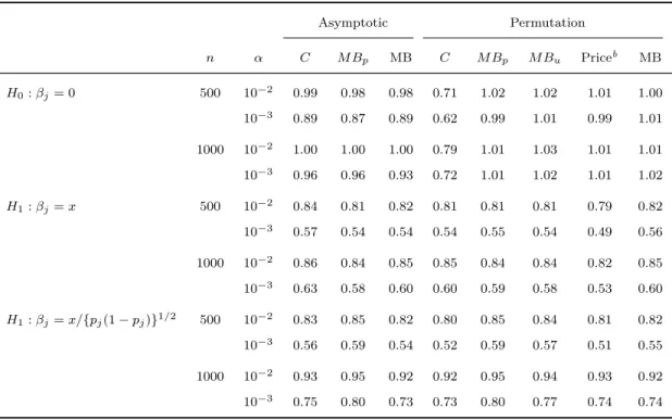
2.2 Type I errora_{and power of asymptotic and}

per-mutation methods . . . 38

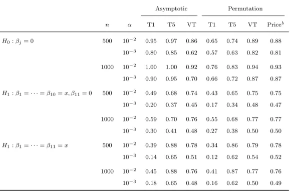
2.3 Type I errora_{and power of fixed and variable}

threshold methods . . . 39

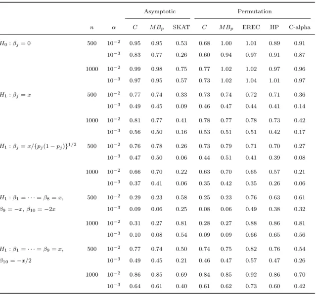
2.4 Type I errora_{and power of asymptotic and} per-mutation tests for detecting potentially opposite

effects . . . 40

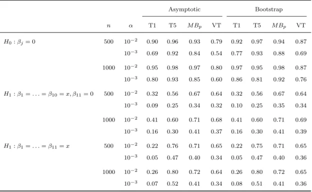
2.5 Type I errora_{and power of fixed and variable}

threshold methods with covariates . . . 41

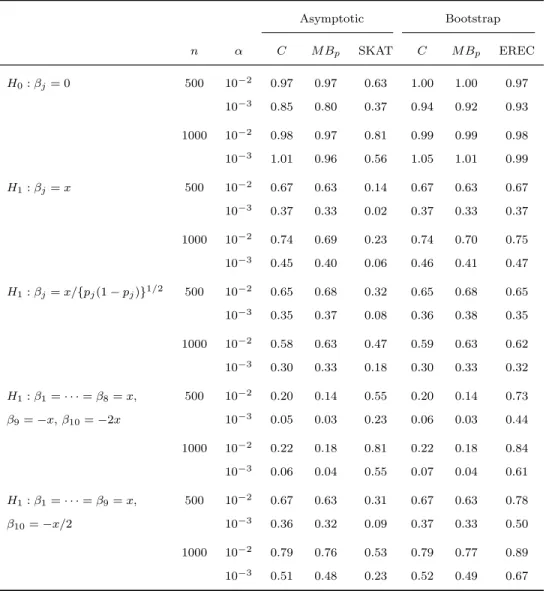
2.6 Type I errora_{and power of asymptotic and} boot-strap tests for detecting potentially opposite

ef-fects in the presence of covariates . . . 42

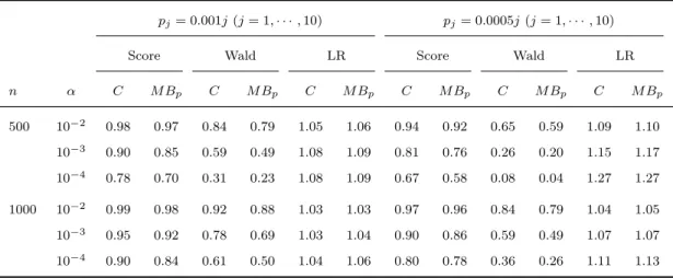
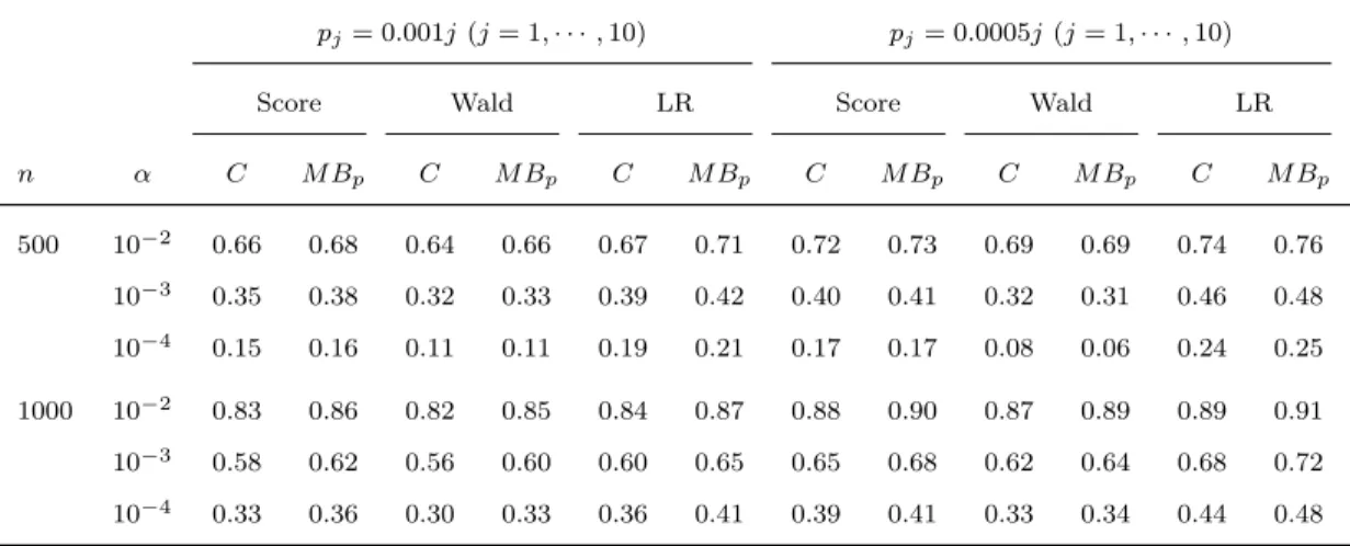
2.7 Type I errora_{and power of asymptotic} meth-ods with different weight functions under pj =

0.0005j (j = 1,· · · ,10) . . . 43 2.8 Type I erroraand power of asymptotic

meth-ods with different weight functions under pj =

0.00025j (j = 1· · · ,20) . . . 43 2.9 Type I errora_{and power of asymptotic methods}

with different weight functions under pj = 0.005

(j = 1,· · · ,10) . . . 44 2.10 Type I errora_{and power of asymptotic}

0.0025 (j = 1,· · · ,10) . . . 44 2.11 Type I errora_{and power of asymptotic}

(10)

2.13 Power of score, Wald and LR tests with

covari-ates under H1 :βj =x (j = 1, . . . ,10) . . . 46

2.14 Power of score, Wald and LR tests with

covari-ates under H1 :βj =x/{pj(1−pj)}1/2 (j = 1, . . . ,10) . . . 46

3.1 Type I erroraat different nominal levels for rare-variant tests based on probit and logistic regres-sions under pj = 0.001j (j = 1,· · · ,10). Bina-ry data are simulated using a logistic regression

model. . . 65

3.2 Type I errora_{at different nominal levels for} rare-variant tests based on probit and logistic regres-sions under pj = 0.01j (j = 1,· · · ,10). Bina-ry data are simulated using a logistic regression

model. . . 66

4.1 Type I error divided by the nominal significance

(11)

LIST OF FIGURES

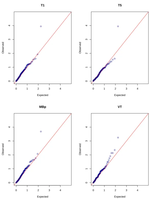
2.1 Quantile-quantile plots of −log₁₀(p-values) for the asymptotic T1, T5, M Bp and VT tests in

the quantitative trait analysis of total cholesterol. . . 50

2.2 Quantile-quantile plots of −log₁₀(p-values) for the permutation EREC, T5, M Bp and VT tests

in the quantitative trait analysis of total cholesterol. . . 51

2.3 Quantile-quantile plots of −log₁₀(p-values) for the asymptotic T1, T5, M Bp and VT tests in

the binary trait analysis of total cholesterol. . . 52

2.4 Quantile-quantile plots of −log₁₀(p-values) for the bootstrap EREC, T5, M Bp and VT tests in

the binary trait analysis of total cholesterol. . . 53

2.5 Quantile-quantile plots of −log₁₀(p-values) for the SKAT in the quantitative and binary trait analyses of total cholesterol (with covariates) and for the SKAT and C-alpha in the binary trait

analysis of total cholesterol without covariates. . . 54

2.6 Quantile-quantile plots of −log₁₀(p-values) for the asymptotic T1, T5,M Bpand VT tests in the

binary trait analysis of total cholesterol without covariates. . . 55

2.7 Quantile-quantile plots of −log₁₀(p-values) for the permutation EREC, T5, M Bp and VT tests in the binary trait analysis of total cholesterol

without covariates. . . 56

2.8 Quantile-quantile plots of −log₁₀(p-values) for the Han-Pan test, Price et al.’s VT test, and the asymptotic and permutation versions of the MB test in the binary trait analysis of total

(12)

3.1 Type I error rates for the ML and na¨ıve methods for detecting genetic associations when the ge-netic effects are positive. The results for the bur-den, VT, and VC tests are shown in the upper, middle, and lower rows, respectively. The left panel shows the power as a function of the ge-netic effect on the primary trait when the corre-lation between the primary and secondary trait-s itrait-s 0.4. The right panel trait-showtrait-s the power atrait-s a function of the correlation between the primary and secondary traits when the genetic effect on

the primary trait is 0.4. . . 69

3.2 Power of the ML and na¨ıve methods for detect-ing genetic associations when the genetic effects are positive. The results for burden, VT, and VC tests are shown in the upper, middle, and lower rows, respectively. The left panel shows the power as a function of the genetic effect on the primary trait when the correlation between the primary and secondary traits is 0.4. The right panel shows the power as a function of the correlation between the primary and secondary traits when the genetic effect on the primary

trait is 0.4. . . 70

3.3 Power of the ML and na¨ıve methods for detect-ing genetic associations when the genetic effects are negative. The results for burden, VT, and VC tests are shown in the upper, middle, and lower rows, respectively. The left panel shows the power as a function of the genetic effect on the primary trait when the correlation between the primary and secondary traits is 0.4. The right panel shows the power as a function of the correlation between the primary and secondary traits when the genetic effect on the primary

(13)

3.4 Power of the meta-analysis using the ML and na¨ıve methods for detecting genetic association-s. The results for the burden, VT, and VC tests are shown in the upper, middle, and lower rows, respectively. For the left panel, we set the ge-netic effect on the primary trait in both studies to 0.4 and the correlations between the prima-ry trait and the secondaprima-ry trait in Study I and Study II to 0.6 and -0.6, respectively. For the right panel, we set the correlations between the primary trait and the secondary trait in both studies to 0.4 and the genetic effect on the pri-mary trait in Study I and Study II to 0.6 and

-0.6, respectively. . . 73

3.5 Quantile-quantile plots for the ML, na¨ıve-M’,

and na¨ıve-C’ meta-analysis results. . . 75

3.6 Pair plots between the p-values for the ML method

and the na¨ıve methods. . . 76

4.1 Power as a function of the between-study het-erogeneity for the quantitative trait. The left, middle and right panels correspond to three dif-ferent genetic structures: (a) genetic effects ex-hibit at the burden score level for variants with MAFs< 5%, (b) genetic effects exhibit at the burden score level for variants with MAFs<1%, and (c) genetic effects exhibit at the individual variant level. For each structure, 80%, 50% or 20% of the variants in ten 300 base-pair regions

were randomly selected to be potentially causal. . . 87

4.2 Power as a function of the between-study hetero-geneity for the binary trait. The left, middle and right panels correspond to three different genetic structures: (a) genetic effects exhibit at the bur-den score level for variants with MAFs<5%, (b) genetic effects exhibit at the burden score level for variants with MAFs<1%, and (c) genetic ef-fects exhibit at the individual variant level. For each structure, 80%, 50% or 20% of the vari-ants in ten 300 base-pair regions were randomly

(14)

4.3 Power as a function of the number of studies with genetic effects on the quantitative trait. The upper, middle and lower panels correspond to three different genetic structures: (a) genet-ic effects exhibit at the burden score level for variants with MAFs<5%, (b) genetic effects ex-hibit at the burden score level for variants with MAFs< 1%, and (c) genetic effects exhibit at the individual variant level. For each structure, 50% of the variants in ten 300 base-pair regions

were randomly selected to be potentially causal. . . 89

4.4 Meta-analysis of the eleven studies in the NHLBI ESP: the left and middle panels are the quantile-quantile plots for the FE and RE tests, and the right panel compares the RE and FE results.

The red dot indicates the gene LDLR. . . 93

4.5 Forest plots for the burden tests with two MAF thresholds for the gene LDLR in the NHLBI E-SP. For each study, the estimate of the genet-ic effect is shown by the square and the corre-sponding 95% confidence interval is shown by the line. The meta-estimate of the genetic effect and the corresponding 95% confidence interval

are shown by the diamond. . . 94

4.6 Standardized LDL values for the carriers of the LDLR mutations in the NHLBI ESP. Each point represents an individual who carries a mutation. There are 54 polymorphic sites with the chr:position IDs and MAFs labeled on the x-axis. The vari-ants are ordered by the MAFs. The vertical line pertains to the MAF threshold at which the test statistics of FE-VT and RE-VT are maximized. The five phenotype groups are indicated by d-ifferent colors. AA and EA subjects are shown in circles and triangles, respectively. The hor-izontal line pertains to the average LDL value

(15)

CHAPTER1: LITERATURE REVIEW

1.1 Introduction

Complex diseases, such as cancer, hypertension, and diabetes, are determined by

a variety of genetic and environmental factors, as well as their interactions. Genetic

dissection of complex human disease is typically accomplished using data from

large-scale genetic association studies, which explore relationship between genetic variants

and disease phenotypes. Biological and empirical evidence suggests that rare variants

account for a significant proportion of the genetic contribution to complex human

diseases. Recent technological advances in next-generation sequencing (NGS) platforms

have made it possible to generate comprehensive information on rare variants in large

samples. Indeed, the number of sequencing studies has been increasing dramatically

due to the widespread availability of NGS technologies and decrease in costs.

Gene-level testing is widely used in rare-variant association studies; however, the

analytical methods must be tailored for different outcomes and study designs. In

ad-dition, the use of asymptotic approximations to assess the statistical significance has

notable limitations in the setting of rare-variant testing. For instance, due to the low

frequency of rare variants, asymptotic approximation may be violated, which can lead

to inflated type I error and loss of power. Furthermore, the analytical distribution

of the test statistic may not be known, and so, the statistical significance has to be

evaluated empirically. Valid resampling methods for gene-level tests would therefore

(16)

Although next-generation sequencing is much more cost-effective than Sanger

se-quencing, it is not economically feasible to sequence all study subjects in a very large

cohort. A cost-effective strategy is to sequence only those subjects with extreme

val-ues of a quantitative trait. In the National Heart, Lung, and Blood Institute Exome

Sequencing Project (NHLBI ESP), subjects with the highest or lowest values for body

mass index (BMI), low-density lipoprotein (LDL), or blood pressure (BP) were

select-ed for whole-exome sequencing. Failure to account for such trait-dependent sampling

can cause severe inflation of type I error and substantial loss of power in quantitative

trait analysis, especially when combining results from multiple studies that used

differ-ent selection criteria. Thus, the valid and efficidiffer-ent statistical methods are needed for

rare-variant association testing under such sampling design.

Due to the limited carriers of the rare mutations and high background rates of

neutral variation even in causal genes, a single study is often underpowered to identify

rare variants. Thus, meta-analysis becomes an important tool to increase statistical

power by combining summary statistics over multiple studies. Fixed-effects models

have been adopted almost exclusively for meta-analysis in genetic research. However,

fixed-effects methods lose power if gene-level associations are heterogeneous among

studies.

In this proposal, we first conduct a literature review in Chapter 1. In Chapter

2, we introduce a general framework for gene-level association analysis and develop

asymptotic and resampling methods for different traits and study designs. In Chapter

3, we investigate a maximum likelihood framework to analyze binary secondary traits

under trait-dependent sampling. Finally, in Chapter 4, we propose methods for

(17)

1.2 Gene-level association tests

Genome-wide association studies (GWAS) using tagSNPs (representative single

nu-cleotide polymorphism in a region of the genome) have successfully identified common

SNPs with small to modest effects for virtually every complex human disease. The

standard approach for analyzing GWAS data is to apply a univariate test at each

vari-ant and then assess significance by using an appropriate p-value threshold, taking into

account multiple testing. For dichotomous disease traits, commonly used association

tests include χ2 _{test, Fisher’s exact test, alleles test, Armitage trend test, and tests}

based on logistic regression. The χ2 _{test and Fisher’s exact test can be employed for}

testing recessive, dominant, or codominant modes of inheritance. The alleles test and

the Armitage trend test are tests of the additive mode of inheritance, in which the

geno-types 0/1/2 are viewed as ordered categories. The regression approach is more flexible

because it allows for covariate adjustment (e.g., principle components, environmental

factors, and interactions) and different types of phenotypes (e.g., dichotomous disease

indicator, count, or continuous measurement).

Genetic association studies may test hundreds of thousands of genetic variants for

association with disease. Failure to account for the effects of multiple comparisons may

result in an abundance of false positive results. Several approaches have been developed

to correct for multiple testing. The simplest approach is to use a Bonferroni correction.

In a typical GWAS study, thep-value cutoff for declaring significance is 5×10−8. This figure is based on the approximate number of independent common variants across the

genome. However, the Bonferroni correction is highly conservative, especially when the

variants are in strong linkage disequilibrium. Permutation and Monte-Carlo methods

(Lin 2005) are common alternative approaches to control false positive rates.

(18)

for disease association with multiple variants simultaneously. Such tests not only

cap-ture the linkage disequilibrium patterns, but also decrease the number of required tests

and thus reduce the penalty for multiple testing. The multivariate approach may be

more powerful than the single-variant test if the variants have moderate effect sizes.

Commonly used multivariate tests include Hotelling’s T2 _{test and multivariate tests}

based on regression. However, the large degrees of freedom compromise the power of

these tests. In addition, simulation shows that Hotelling’sT2 test is highly sensitive to

allele frequencies and power reduces drastically when the number of variants increase

(Li and Leal 2008).

Technological advances in NGS platforms have made it possible to extend

associa-tion studies to rare variants in targeted exons and eventually, the entire genome. Rare

variants are believed to be enriched for functional alleles and have stronger effects on

complex diseases than common variants (Pritchard 2001, Gorlov et al. 2008). Indeed,

deep-resequencing studies of candidate genes have already demonstrated the influence

of rare variants on several complex traits (Cohen et al. 2004, Ahituv et al. 2007,

Nejent-sev et al. 2009). Single-variant analysis has limited power in rare-variant association

studies because only a small percentage of study subjects carry a rare mutation and

ad-justments need to be made for multiple testing. Other methods have been developed for

detecting rare-variant associations (Tzeng and Zhang 2007, Li and Leal 2008, Madsen

and Browning 2009, Han and Pan 2010, Liu and Leal 2010, Price et al. 2010, Wu et al.

2011, Sun et al. 2013). These methods are usually called “gene-level” methods because

they combine information across multiple variant sites within a gene and the tests are

performed for individual genes instead of individual variants. The gene-level methods

can enrich association signals and reduce the penalty for multiple testing. In addition,

prior biological knowledge (e.g., variant function, deleterious prediction) can be used to

(19)

of different gene-level methods.

1.2.1 Burden tests: CAST, GRANVIL, CMC

The burden tests generate genetic variable(s) by collapsing variants on the basis of

specific criteria and applying univariate or multivariate tests for analysis of the genetic

variable(s). The commonly-used criterion is to aggregate variants with minor allele

frequencies (MAFs) less than a certain frequency threshold, and most burden tests are

based on one genetic variable. For example, the Cohort Allelic Sums Test (CAST)

collapses all variants below some frequency threshold and contrasts the number of

individuals with one or more mutations between cases and controls (Morgenthaler and

Thilly 2007). The Gene- or Region-based ANanlysis of Variants of Intermediate and

Low frequency test (GRANVIL) is another burden test similar to CAST, in which

the likelihood ratio test is performed under a linear regression framework (Morris and

Zeggini 2010).

The CAST and GRANVIL tests enrich the association signals and reduce the

num-ber of degrees of freedom for testing. However, the inclusion of non-causal variants or

the exclusion of causal variants during collapsing dilutes the association signal and

ad-versely affects the power. The Combined Multivariate and Collapsing (CMC) test was

developed to harness the advantages of both the collapsing and multivariate tests (Li

and Leal 2008). For the CMC test, variants are divided into rare and common groups

based on an allele frequency cutoff. In particular, rare variants (e.g., those with MAFs

<0.01) are collapsed together, whereas each common variant forms a separate group.

Within each group, the individuals are coded as 1 if they carry one or more mutations

and coded as 0 otherwise. A multivariate test (e.g., Hotelling’sT2 _{test) is then applied}

for detecting diseases associated with those genetic variables. The CMC test is more

(20)

collapsing methods. In addition, the CMC test has the advantage of allowing both rare

and common variants to contribute to the overall test for the effect of a gene, although

a large number of degrees of freedom are required when testing many common variants.

1.2.2 Weighted approach: WSS, KBAC

The CMC test depends on the ad hoc choice of a frequency cutoff to distinguish

rare and common variants. The weighted approach, on the other hand, aggregates rare

and common variants and assigns different weights to each group. In the weighted

approach, the genetic variable for an individual is calculated as a weighted sum of the

mutation counts. This approach accentuates signals from rare mutations such that the

test is not completely dominated by common mutations. The Madsen and Browning

method weights each mutation according to its frequency in the unaffected subjects and

permutes the disease status to assess the significance of a Wilcoxon-type test statistic

(Madsen and Browning 2009). In the Kernel-Based Adaptive Cluster (KBAC) method,

the weight is based on the kernel functions, depending on the estimated sample risk,

and the permutation procedure is applied to evaluate the significance of the score test

statistics under a logistic regression model (Liu and Leal 2010).

1.2.3 Maximization approach: VT

The optimal choice of the MAF cutoff depends on the true disease model, which

is unknown. In addition, a variant with frequency 0.01 is rare in a small data set of

500 individuals but is quite common in a much larger data set of 100,000 individuals.

Therefore, a fixed-threshold may not be appropriate for all diseases and data sets. The

variable threshold (VT) test developed by Price et al. (2010) uses the maximum of

the test statistics over all unique allele-frequency thresholds and assesses statistical

(21)

allele-frequency thresholds and different weight functions.

1.2.4 Signed approach: Han and Pan

The foregoing tests do not have good power if the variants being combined have

opposite effects on the phenotype. Several other tests aim to detect variants with

opposite effects. The methods proposed by Han and Pan incorporate the signs of the

observed effects into the calculation of the genetic variables and apply a permutation

procedure to assess the significance (Han and Pan 2010). This test was motivated by

the data-adaptive modifications to an aggregation test originally proposed for common

variant analysis, which aims to strike a balance between utilizing information from

multiple markers in linkage disequilibrium and reducing the cost of large degrees of

freedom or adjustments for multiple testing.

1.2.5 Variance-Component (VC) tests: Similarity regression, C-alpha, SKAT

VC tests are aimed at detecting variants with opposite effects within a gene. VC

tests can be motivated from the similarity regression or kernel-machine regression.

In these regression frameworks, the genetic effects are incorporated into the model

through a nonparametric function h(Gi1, . . . , GiK), where Gik is the genotype of the

kth variant for the ith subject. Supposed Gi = (Gi1, . . . , GiK), then the form of the

nonparametric function is determined by a user-specified, positive, semi-definite kernel

matrix K(Gi, Gj), which measures the genomic similarity between the genotypes of

the ith and jth subjects. Some commonly used kernels include (weighted) linear,

identity-by-descent, and quadratic kernels. By the representation theory, h(Gi) can

be written as Pn

j=1αjK(Gi, Gj) with parameters α1, . . . , αn. It can be shown that this nonparametric regression framework is equivalent to the random-effects model

(22)

τ K. Therefore, testing h = 0 is equivalent to testing τ = 0. Based on the working

random-effects model, the score test statistic can be constructed, and the asymptotic

distribution can be derived. A related test is SKAT-O, which is a weighted sum of the

burden and VC statistics (Lee et al. 2012).

1.3 Trait-dependent sampling

The rare variants that are involved in complex trait etiologies usually only have

moderate effect sizes, and even their aggregated frequencies across a genetic region can

be limited. Therefore, a large number of samples must be sequenced and analyzed in

order to have adequate power to detect associations. Although NGS is much more

cost-effective than Sanger sequencing, it is still expensive to generate high read depth

data for a large number of samples. To reduce expenses and increase statistical power

of association tests, many sequencing projects select samples based on the value of

a trait of primary interest (i.e., the primary trait). Indeed, previous research shows

that trait-dependent sampling can substantially increase power comparing to random

sampling with equal sample sizes. In the NHLBI ESP, multiple studies were included,

each of which was focused on one primary trait. Subjects with extreme high or low

values of the quantitative primary traits BMI, LDL and BP were selected for

whole-exome sequencing. For the binary primary traits myocardial infarction (MI) and stroke,

case-control (MI) and case-only (stroke) samples were generated for sequencing. In

addition, a large random sample was created and referred to as the deeply phenotype

reference (DPR). In addition to the primary trait, there were many quantitative and

binary secondary traits across the six studies (e.g, high-density lipoprotein, triglyceride,

diabetes). A mega- or meta-analysis that includes these secondary traits would boost

(23)

However, the trait-dependent sampling study design produces challenges for

ana-lyzing secondary traits. If the secondary trait is correlated with the primary trait, and

the primary trait is associated with a genetic variable, then spurious secondary trait

association will be created among the subjects with extreme values of the primary trait.

Thus, standard methods that ignore the sample ascertainment yield biased effect

esti-mates and inflated type I error in association tests. For quantitative secondary traits,

the properties of the na¨ıve methods have been investigated theoretically and empirically

(Lin et al. 2013). In the subsequent materials, we show the likelihood-based methods

and the three types of gene-level tests that have been developed.

Suppose that we have a cohort of n subjects, among whomn1 subjects are selected

for sequencing. We assume that the primary trait Y1 is available on all n cohort

members. (If there are missing values onY1, we define n as the total number of subjects

with available Y1.) The selection of subjects for sequencing may depend on the values

of Y1 in the entire cohort. By definition, the genotype G is available only on the n1

sequenced subjects. We assume that the covariate Z and the secondary trait Y2 are

available only on the n1 sequenced subjects. The values of Y2 may be missing among

the sequenced subjects.

We allowGandZto differ between the primary and secondary traits. The

observed-data likelihood can be expressed as

n1

Y

i=1

P(Y1i|G1i, Z1i)P(G1i, Z1i)

n

Y

i=n1+1

X

g,z

P(Y1i|g, z)P(g, z)

n2

Y

i=1

P(Y2i|Y1i, G2i, Z2i). (1.1)

It is natural to formulate the joint distribution of Y1 and Y2 through the bivariate

linear regression model:

(24)

whereG1 andG2 may pertain to individual variants or (weighted) burden scores.

Con-ditioned onY1,Y2 satisfies the following linear regression model:

Y2 =δYe₁+β₂TG₂+γ₂TZ₂ +

e

2,

whereYe1 =Y1−β1TG1−γ1TZ1.

1.3.1 Estimating parameters for the primary trait

We maximize the first two terms in expression 1.1 to obtain the maximum likelihood

estimates (MLEs) of (β1, γ1, σ11) and P(·,·). We adopt the nonparametric maximum likelihood estimation (NPMLE) approach to estimate P(·,·) by the discrete proba-bilities at (g1, z1),· · · ,(gm, zm), which are the distinct observed values of (G1i, Z1i)

(i = 1, . . . , n1). We denote the point mass at (gj, zj) as qj. Then, we maximize the

following objective function

n1

X

i=1

"

logP(Y1i|G1i, Z1i) + log m

X

j=1

I{(G1i, Z1i) = (gj, zj)}qj

#

+ n

X

i=n1+1

log m

X

j=1

P(Y1i|gj, zj)qj,

whereI{·}is the indicator function.

The maximization is carried out through an expectation-maximization (EM)

al-gorithm, in which the missing values of (G1, Z1) for the non-sequenced subjects are

inferred from the discrete probability distribution with point mass qj at (gj, zj) (j =

1,· · · , m). Start with the initial values:

β1 = 0, γ1 = 0, σ11 = sample variance of Y1 based on (Y11, . . . , Y1n),

and qj = 1/m, j = 1, . . . , m.

(25)

E-step. For i = 1, . . . , n1, we set ψij = I{(G1i, Z1i) = (gj, zj)}. For i = n1 + 1, . . . , n, we set

ψij =

P(Y1i|gj, zj)qj

Pm

k=1P(Y1i|gk, zk)qk

,

whereP(y1|g, z) = (2πσ11)−1/2exp{−(y1−β1Tg−γ1Tz)2/(2σ11)}.

M-step. We update the parameter values as follows:

η= n X i=1 m X j=1

ψijWjWjT

!−1 _n

X i=1 Y1i m X j=1

ψijWj

!

and

σ11=n−1

n X i=1 m X j=1

ψij(Y1i−ηTWj)2,

where η=    β1 γ1  

 and Wj =    gj zj   . In addition,

qj =n−1

n

X

i=1

ψij, j = 1,· · · , m.

At convergence, we obtain the estimator (βb₁, b

γ1,bσ11,qb1, . . . ,qbm). It follows from

Theorem 1 of Lin and Zeng (2006) that the estimator is consistent, asymptotically

normal ,and asymptotically efficient. We estimate the asymptotic covariance matrix

according to the Louis formula. For i = 1, . . . , n and j = 1, . . . , m, let l1ij and l2ij be

the first and second derivatives, respectively, of logP(Y1i|gj, zj) + logqj with respect to

(β1, γ1, σ11, q1, . . . , qm). We then calculate the information matrix as

Q1 =−

n X i=1 m X j=1

ψijl2ij −

n X i=1    m X j=1

ψijl1ijl1ijT −

m

X

j=1

ψijl1ij

! _m X

j=1

ψijl1ij

!T  

.

To account for the constraint that Pm

(26)

matrix of (β1, γ1, σ11, q1,· · · , qm) with respect to (β1, γ1, σ11, q1,· · · , qm−1). Then, the asymptotic covariance matrix of the estimator (βb1,bγ1,σb11,bq1,· · · ,qbm−1) is estimated by

Ω1 =F−1, whereF =DTQ1D.

1.3.2 Estimating parameters for the secondary trait

To estimate (δ, β2, γ2,σe22), we maximize the last term in (2.1) or equivalently apply

the standard least-squares method to the observations (Y2i,Yb_1i, G_2i, Z_2i) (i= 1, . . . , n₂),

whereYb1i =Y1i−βb₁TG1i−bγ

T

1Z1i. That is,

      b δ b β2 b γ2       =       n2 X i=1       b Y1i G2i Z2i      

⊗2

    

−1_

     n2 X i=1 Y2i       b Y1i G2i Z2i             and b e

σ22=n−21

n2

X

i=1

(Y2i−bδYb_1i−βb₂TG_2i− b

γ₂TZ2i)2,

wherea⊗2 ₌_aaT_{. We estimate the covariance matrix of (}

b

δ,βb₂,

b

γ2) by

Ω2 =b e σ22       n2 X i=1       b Y1i G2i Z2i      

⊗2

     −1

+JΩe₁JT,

whereJ is the Jacobian matrix of (δ,b βb₂, b

γ2) with respect to (βb₁, b

γ1), andΩe₁ is the block

of Ω1 corresponding to (β1, γ1).

1.3.3 Performing association tests

To calculate the score statistic for testing the null hypothesisH₀(1) :β1 = 0, we

calcu-late the restricted MLE of (γ1, σ11, q1,· · · , qm) underH (1)

(27)

the aforementioned EM algorithm, in which β1 is set to 0 and only (γ1, σ11, q1,· · · , qm) is estimated. The score statistic for testingH₀(1) :β1 = 0 is

U1 =

n

X

i=1 m

X

j=1

ψijl

(1) 1ij,

where l_1ij(1) is the component of l1ij corresponding to β1. It can be shown that U1 is

approximately multivariate normal with mean 0 and covariance matrix

V1 =F11−F12F22−1F21,

where

  

F11 F12

F21 F22

 

 is the partition of F forβ1 versus the other parameters.

We test H₀(1) using the quadratic form

U₁TV₁−1U1,

which is referred to theχ2

ddistribution, wheredis the dimension ofβ1. We also consider the maximum test statistic

Tmax = max j=1,...,d|Tj|, where Tj = U1j/V

1/2

1j , U1j is the jth component of U1, and V1j is the jth diagnonal element ofV1. Thep-value ofTmaxis determined by the multivariate normal distribution

of U1. Finally, we consider the weighted quadratic form

Q=UTW U,

whereW is a diagonal matrix of weights that depend on the MAFs through a beta

func-tion. The null distribution ofQis approximated byPd

j=1λjχ 2

(28)

the eigenvalues ofV₁1/2W V₁1/2, and (χ2

1,1, . . . , χ21,d) are independentχ21 random variables.

To test the null hypothesis H₀(2):β2 = 0, we estimate δ, γ2 and σe22 under β2 = 0:

   b δ b γ2   =    n2 X i=1    b Y1i Z2i   

⊗2

 

−1_

  n2 X i=1 Y2i    b Y1i Z2i       and b e

σ22=n−21

n2

X

i=1

(Y2i−bδYb_1i− b

γ₂TZ2i)2.

We calculate

U2 =b

e

σ−₂₂1

n2

X

i=1

(Y2i−bδYb_1i− b

γ₂TZ2i)G2i,

which is approximately multivariate normal with mean 0 and covariance matrix

V2 =b

e

σ−₂₂1

       n2 X i=1

G⊗_2i2−

   n2 X i=1 G2i    b Y1i Z2i    T      n2 X i=1    b Y1i Z2i   

⊗2

 

−1_

  n2 X i=1    b Y1i Z2i   G T 2i          

+BΩe₁BT,

where B is the Jacobian matrix of U2 with respect to (βb₁,_bγ₁). We test H

(2)

0 by using the aforementioned three types of test statistics.

1.4 Meta-analysis

1.4.1 Meta-analysis of GWAS

GWAS have successfully identified common SNPs with small to modest effects for

virtually every complex human disease (Hardy and Singleton 2009). For variants with

(29)

small sample size. Meta-analysis is an important tool to combine evidence from

mul-tiple studies and explain part of the missing heritability that was not easy to capture

in individual studies. Many new findings have been made through meta-analysis of

GWAS (Saxena et al. 2007, Scott et al. 2009, Franke et al. 2010). Fixed-effects models

have been adopted almost exclusively; these models assume a common genetic effect

across studies. Multiple meta-analysis methods for GWAS have been developed and

are described below.

1. p-value-based methods

Let pk denote the p-value from the kth study among a total of K studies. Assuming

that theK studies are independent, the simplest meta-analysis approach is to combine

the p-values using Fisher’s method

T =−2

K

X

k=1

log(pk)

or Stouffer’s method

Z =

PK

k=1Zkwk

q PK

k=1w2k

,

wherewk is the square root of the sample size of the kth study, and

Zk = (sign for effect direction)∗Φ−1

1−pk

2

,

where Φ(·) is the cumulative density function for the standard normal distribution. The major disadvantage of the p-value-based meta-analysis method is that it can not

provide an overall estimate of the effect size.

(30)

Let X1,· · · , XK denote the estimate of the effect sizes for the K studies. Inverse-variance weighting is usually applied to estimate overall genetic effect under fixed-effects

models. The overall effect size estimate takes the form

X =

PK

k=1wkXk

PK

k=1wk

,

wherewk is the inverse of the variance forXk. The variance of the estimate is

var(X) = 1

PK

k=1wk

.

3. Bayesian methods

Some consortia have applied Bayesian approaches for meta-analysis. For example, the

Wellcome Trust Case Control Consortium has used the Bayes factor that represents the

ratio of the probability of the data under the null hypothesis to the probability of the

data under the alternative hypothesis. Bayesian models are intuitive, but the result

may depend on the assumptions about the prior distribution, and the genome-wide

im-plementation can be computationally intensive. It has been shown that Bayes factors

and p-values often yield similar rankings for common variants. However, differences

can be observed for rare or low-frequency variants (Wakefield 2009).

4. Methods that account for between-study heterogeneity

An alternative approach is the random-effects model in which the genetic effect is

allowed to be heterogenous among studies. There are multiple sources of heterogeneity

across genetic studies: populations with different demographic features (Waters et al.

(31)

et al. 2009, Tobacco and Consortium 2010); and inconsistencies in data collection and

manipulation (Ioannidis et al. 2007) (e.g., genotyping platforms, quality control criteria,

or imputation methods). Nevertheless, the random-effects model is seldom used in

genetic association studies for two reasons: (1) The random-effects model requires a

large number of studies to make valid asymptotic inference, but the number of available

genetic association studies is usually small. (2) The conventional test under the

random-effects model gives less significantp-values than the corresponding test under the

fixed-effects model. In a recent paper by Han and Eskin (2011), this phenomenon was

described, and the cause was discovered to be the implicit assumption of heterogeneity

under the null hypothesis that the variant is not associated with the trait of interest.

A new test was proposed in their paper that relaxes this assumption and thus, is more

powerful than the test under the fixed-effects model when heterogeneity exists. To

account for the fact that the number of studies is small, the Monte-Carlo method is

used to obtain thep-value.

1.4.2 Meta-analysis of sequencing studies

We reviewed various level tests in Section 1.1. Three major types of

gene-level tests are the burden, VT, and VC tests. None of these tests is universally most

powerful. The burden and VT tests can outperform the VC test when a large proportion

of the variants are causal and harboring unidirectional effects, whereas the VC tests

tend to be more powerful when a small proportion of the variants are causal and

harboring bidirectional effects. Therefore, it is necessary to develop different

meta-analysis methods for each of these tests. Of course, one can always combine p-values

through the Fisher and Stouffer methods; software that implements this approach has

been developed (e.g., RAREMETAL). However, it has been shown that meta-analysis

(32)

address the heterogeneity issue usingp-values. Tang and Lin (2013) and Liu et al. (2014)

have developed meta-analysis methods that combine score statistics across studies for

gene-level tests under fixed-effects models. We review the fixed-effects methods in the

subsequent materials.

Suppose that we are interested indgenetic variables, which may be the genotypes of

individual variants or the burden scores for a gene. For each ofK studies, we calculate

the (multivariate) score statistic for testing the null hypothesis that none of thedgenetic

variables has any effect on the trait of interest, and we also calculate the corresponding

information matrix. We sum the score statistics and information matrices over the K

studies to obtain the overall score statistic Uand overall information matrix V. Note that U is a d×1 vector and V is a d×d matrix. Under the null hypothesis, U is (asymptotically) multivariate zero-mean normal with covariance matrix V. It can be shown thatUis the score statistic for the common genetic effects in the joint likelihood based on the original data of theK studies, allowing nuisance parameters to be different

among the studies (Lin and Zeng, 2010). Thus, association testing based onU and V

is equivalent to the joint analysis of the original data.

Given Uand V, we perform three types of multivariate tests, which encompass all commonly used rare-variant tests.

1. Quadratic statistic:

Q=UTV−1U.

Under the null hypothesis, Q is distributed as χ2

d. If U pertains to a specific burden score, then Q is a burden test. If U pertains to the genotype values of common SNPs and the burden score of rare variants, then Q is the CMC test (Li and Leal, 2008).

2. Maximum statistic:

Tmax= max j=1,...,dUj

(33)

where Uj is the jth component of U, and Vj is the jth diagonal element of V. The

p-value of Tmax is determined by the multivariate normal distribution of U (Lin and Tang, 2011). If the genetic variables consist of the burden scores at different MAF

thresholds, then Tmax is the VT test. If the genetic variables pertain to different types

of burden scores, thenTmaxcan be used to adjust for multiple testing with those burden

scores.

3. Weighted quadratic statistic:

Qw =UTWU,

whereWis a weight matrix. The null distribution ofQw is determined byPd_j=1λjχ21,j, where λj is the jth eigenvalue of V1/2WV1/2, and χ21,1, . . . , χ21,d are independent χ21 random variables. If the genetic variables are the genotypes of individual SNPs, then

Qw becomes the SKAT or C-alpha test. For the SKAT test, W is a diagonal matrix that depends on the MAFs through a beta function; for the C-alpha test, W is an identity matrix.

These fixed-effects meta-analysis methods lose power if the genetic effects are

het-erogeneous among studies. Recently, Lee et al. (2013) proposed two test statistics to

allow for heterogeneous effects:

Het-SKAT = d

X

j=1 K

X

k=1

w_kj2 S_kj2 and

Het-SKAT-O =%

d X

j=1 K

X

k=1

wkjSkj

2

+ (1−%) d

X

j=1 K

X

k=1

w_kj2 S_kj2 ,

whereSkjis the score statistic for testing thejth variant in thekth study,wkj is a weight

for the jth variant, and % is chosen to minimize the p-value. Het-SKAT is essentially

(34)

average effect size is large or the heterogeneity exhibits at the burden score instead of

the variant level. Het-SKAT-O is a weighted sum of fixed-effects burden test (under the

additive mode of inheritance) and Het-SKAT and thus is a joint test of the mean effect

at the burden score level and the heterogeneity at the variant level. Het-SKAT-O will

lose power if both the mean effects and heterogeneity exhibit at the burden score level

or if both the mean effects and heterogeneity exhibit at the individual variant level.

The p-values of Het-SKAT and Het-SKAT-O are based on asymptotic distributions.

Consequently, the type I error may not be well-controlled, the burden scores can only

be calculated under the additive mode of inheritance, and the same set of weights has

to be used for the two components of Het-SKAT-O.

In Chapter 4, we investigate the performance of the aforementioned meta-analysis

(35)

CHAPTER2: A GENERAL FRAMEWORK FOR DETECTING DISEASE ASSOCIATIONS WITH RARE VARIANTS IN

SEQUENCING STUDIES

2.1 Introduction

In this chapter, we provide a general framework for association testing with rare

variants that reflects the spirits of the existing methods but is statistically more

power-ful and computationally more efficient. Our framework covers all major study designs

(i.e., case-control, cross-sectional, cohort and family studies) and all common

pheno-types (e.g., binary and quantitative traits, and potentially censored ages at onset of

disease) and allows any covariates (e.g., environmental factors and ancestry variables).

The ability to accommodate covariates is critically important because population

strat-ification is expected to be a more severe issue with rare variants than with common

variants but may be corrected by including suitable ancestry variables (e.g., percentage

of African ancestry or principal components for ancestry) in the association analysis.

We combine information across multiple variant sites within a gene by taking a weighted

sum of the mutation counts for each study subject and relate the combined

informa-tion and covariates to disease phenotypes through appropriate regression models. We

derive theoretically optimal weights that would produce the most powerful tests among

all valid tests and develop the corresponding testing procedures. We employ score-type

statistics, which are numerically stable even in the case of extremely rare variants and

computationally fast even in the presence of covariates. We provide asymptotic normal

(36)

and other resampling tests that can accommodate covariates. We investigate

theoreti-cally and numeritheoreti-cally when normal approximation is appropriate and when resampling

is required. We modify the popular methods of Madsen and Browning and Price et

al. to enhance statistical power, avoid permutation and accommodate covariates. We

construct data-adaptive test statistics that are powerful even when the combined rare

mutations have opposite effects on the phenotype. The advantages of the new methods

over the existing ones are demonstrated both analytically and empirically.

2.2 Methods

Suppose that a total of n subjects are genotyped on a total of m SNPs in a gene

and that there are d covariates. Here, the word “gene” refers to the group of variants

that will be collectively analyzed and may pertain to a subset of SNPs within a gene

or to a region/pathway involving multiple genes; “covariates” may include non-genetic

variables, such as age and smoking status, as well as ancestry variables, such as

per-centage of African ancestry and principal components for ancestry. For i = 1, . . . , n,

letYi be the phenotype value of the ith subject; for i = 1, . . . , n and j = 1, . . . , m, let

Xji denote the number of the rare mutation theith subject carries at the jth SNP; for

i = 1, . . . , n and j = 1, . . . , d, let Zji denote the value of the jth covariate on the ith

subject. We can write

Xi =

      X1i .. . Xmi      

, Zi =

         1 Z1i .. . Zdi          .

(37)

2.2.1 Binary phenotypes

It is natural to relateYi toXi and Zi through the logistic regression model:

Pr(Yi = 1) =

eβTXi+γTZi

1 +eβT_X

i+γTZi,

whereβandγ arem×1 and (d+1)×1 vectors of unknown regression parameters. Since the first component of Zi is 1, the first component of γ corresponds to the intercept.

Writeβ =τ ξ, whereτ is a scalar constant, andξ=β/τ. Then equation above becomes

Pr(Yi = 1) =

eτ Si+γTZi

1 +eτ Si+γTZi,

whereSi =ξTXi. Note that ξ= (ξ1, . . . , ξm)T is a m×1 vector of weights and that Si is a weighted linear combination of X1i, . . . , Xmi with Xji receiving the weight ξj. We

will refer to ξ as the weight function.

The score statistic for testing the null hypothesis H0 :τ = 0 takes the form

U =

n

X

i=1

Yi−

eγb

T_Z

i

1 +ebγ

T_Z

i !

Si,

where_bγ is the restricted maximum likelihood estimator of γ, which solves the equation

n

X

i=1

Yi−

eγT_Z

i

1 +eγT_Z

i !

Zi = 0.

The variance of U is estimated by

V =

n

X

i=1

viSi2−

n

X

i=1

viSiZi

!T _n X

i=1

viZiZiT

!−1 _n

X

i=1

viSiZi

!

(38)

where

vi =

ebγ

T_Z

i

(1 +eγb

T_Z

i)2.

Under H0, the test statistic T = U/V1/2 is asymptotically standard normal. In the

absence of covariates,

U =

n

X

i=1

(Yi−Y)Si,

and

V =Y(1−Y)

  

n

X

i=1

S_i2−n−1

n

X

i=1

Si

!2  

,

whereY =n−1Pn

i=1Yi.

The true value of the weight function ξ = (ξ1, . . . , ξm)T is unknown and must be

determined biologically or empirically. If we set ξj = 1 (j = 1, . . . , m), then T is a

burden test, which counts the total number of rare mutations each subject carries over

themSNPs. If we believe that common variants are not associated with the phenotype,

then we set ξj = 0 if pj > c, where pj is the minor allele frequency (MAF) of the jth

SNP, and c is a given threshold. If we set ξj = {pj(1−pj)}−1/2 (j = 1, . . . , m), then the weight function is in the same vein as that of Madsen and Browning.

If the choice of the weight functionξ is not proportional to β orξ is estimated from

the data, then U is no longer the score statistic. However, it is simple to verify that

the test statistic T is asymptotically standard normal under H0 regardless of how ξ is

determined. The only condition is that, if ξ is estimated from the data, the estimate

converges to a constant vector as the sample sizenincreases. This condition is satisfied

by all sensible estimates, including those based on estimated allele frequencies. If the

choice ofξ or the limit of the estimate ofξ is proportional toβ, then the corresponding

test statistic T is the most powerful among all valid tests.

The weight function ξ is similar to that of Price et al. The latter authors showed

(39)

the choice ofξj ={pj(1−pj)}−1/2(j = 1, . . . , m) corresponds to the implicit assumption that log(ORj) ∝ {pj(1−pj)}−1/2 (j = 1, . . . , m), where ORj is the odds ratio in the 2×2 table for thejth SNP. Our theory is much more general in that it assumes unknown allele frequencies and accommodates covariates. Indeed, the proposed test statistic is

optimal ifξis proportional to the set of regression parameters (in the limit); this result

holds for all phenotypes, including binary and continuous traits, as well as potentially

censored ages at onset of disease.

Madsen and Browning suggested to setξj ={pbj(1−pbj)}

−1/2 ₍_j _{= 1}_{, . . . , m}_{), where}

b

pj is the estimate of the MAF of the jth SNP in the unaffected subjects. Because the

weights depends on the phenotype values, the authors suggested a permutation-based

test. Our testing framework allows such data-dependent weights since the

frequen-cy estimates converge to the true values as n increases. To improve the accuracy of

asymptotic approximation, we suggest to estimate the frequencies from all study

sub-jects rather than the unaffected subsub-jects. Because the variants can be very rare, we

recommend to add pseudo counts when estimating the frequencies, as was done by

Madsen and Browning. The weight functions based on the frequency estimates in the

pooled sample and the unaffected subjects will be denoted by “M Bp” and “M Bu”,

respectively; the constant weight function will be denoted by “C”. The corresponding

tests will be referred to as “M Bp-test”, “M Bu-test” and “C-test”.

Although M Bu is the weight function used by Madsen and Browning, our M Bu

-test is fundamentally different from the Madsen and Browning (MB) -test. The latter is

based on the sum of the ranks of theSi’s with weight function M Bu over the affected

subjects. Madsen and Browning proposed to assess the statistical significance of their

rank-sum statistic by permutation. They also suggested an asymptotic normal

(40)

Because the mean and standard derivation are estimated by permutation, the

asymp-totic version of the MB test is many orders of magnitudes slower than our asympasymp-totic

tests. The rank-sum statistic is confined to case-control analysis without covariates.

Price et al. developed a VT method by taking the maximum of the test statistics

(i.e., z-scores) over all allele-frequency thresholds and assessing statistical significance

by permutation. We describe below a more general approach that allows not only

multiple allele-frequency thresholds but also different types of weight function; it also

accommodates covariates and does not require permutation.

We considerK choices ofξ, which may correspond to different thresholds or different

types of weight function, or both. For the kth choice of ξ, the corresponding Si is

denoted bySki. Then the “score” statistic is

Uk =

n

X

i=1

Yi−

ebγ

T_Z

i

1 +ebγ

T_Z

i !

Ski,

and the test statistic is Tk =Uk/V 1/2

k , where

Vk=

n

X

i=1

viSki2 −

n

X

i=1

viSkiZi

!T _n X

i=1

viZiZiT

!−1 _n

X

i=1

viSkiZi

!

.

We can show that, under H0, the random vector (U1, . . . , UK)T is approximately K

-variate normal with mean 0 and covariance matrix {Vkl;k, l= 1, . . . , K}, where

Vkl =

n

X

i=1

viSkiSli−

n

X

i=1

viSkiZi

!T _n X

i=1

viZiZiT

!−1 _n

X

i=1

viSliZi

!

.

For the two-sided test, we consider the maximum of the absolute test statistics

(41)

Lettmax be the observed value of Tmax. The p-value is given by

Pr(Tmax≥tmax) = 1−Pr(|T1|< tmax, . . . ,|TK|< tmax),

which is evaluated by treating (T1, . . . , TK)T as aK-variate normal random vector with

mean 0 and covariance matrix {rkl;k, l = 1, . . . , K}, where rkl =Vkl/(VkkVll)1/2. (The one-sided p-value can be calculated in a similar manner.) We reject H0 if the p-value

is smaller than the nominal significance levelα.

The tests based on positive weight functions, such as C, M Bu and M Bp, will have

low power if the mutations being combined have opposite effects on the phenotype. The

optimal choice ofξjisβj, which is unknown. We can estimateβjfrom the data. It would

be tempting to set ξj to βb_j, where βb_j is an appropriate estimate of β_j. There are two

major problems with this strategy. First, the test statisticT will not be asymptotically

normal. Second, theβbj’s are highly variable (since the individual variants are very rare)

and can be quite different from the true values of the βj’s. As a compromise, we set

ξj =βb_j+δ, where δ is a given constant. We refer to this weight function as “EREC”,

an abbreviation of estimated regression coefficients. The corresponding test statistic

T will be asymptotically standard normal as long as δ is non-zero. Indeed, the EREC

test is asymptotically optimal in that ξj will converge to βj if we let δ decrease to 0

as the sample size n increases to∞. The asymptotic normality and optimality require large samples. For small samples, we recommend to use a relatively large value ofδ so

that the weights are not unduly driven by the highly variableβb_j’s.

The Han and Pan (HP) statistic is a special case of our score statisticU (for binary

traits without covariates) in which ξj = −1 if βb_j < 0 and the corresponding p-value

<0.1 and ξj = 1 otherwise. The SKAT statistic of Wu et al. is a weighted sum of the

squared score statistics for individual variants, and the C-alpha statistic of Neale et al.

(42)

HP, C-alpha and SKAT tests are not asymptotically optimal.

Because the asymptotic approximation may not be accurate in small samples,

es-pecially when the weight functionξ involves the phenotype valuesYi’s, we also provide

permutation-type tests. In the absence of covariates, we simply permute the phenotype

values Yi’s and calculate the test statistic T for each permutation. Note that it is

nec-essary to re-calculate theSi’s after permuting theYi’s if the weight functionξ depends

on theYi’s.

Our permutation differs from that of Price et al. in that we permute T whereas

they permuted Pn

i=1YiSi. The former is a pivotal statistic whereas the latter is not. (It is desirable to permute a pivotal statistic.) If the test is one-sided and the weight

function does not depend on the phenotype values, then our permutation is equivalent

to Price et al.’s; otherwise, the two are different. For VT methods, the numerators in

the z-scores of Price et al. are the same as ours, but the denominators are not the

same as or proportional to ours. Thus, the permutationp-values are generally different

between the two methods. The permutation version of the MB test requires ranking

the Si’s for each permutation and is thus substantially slower than our permutation

tests.

In the presence of covariates, it is not appropriate to permute the Yi’s because Yi is

generally correlated withZi. Instead, we generate Yi∗ from the fitted null model:

Pr(Y_i∗ = 1) = e

b γT_Z

i

1 +ebγ

T_Z

i,

and replace theYi’s with theYi∗’s to calculate the test statistic. This process is repeated

and is called (parametric) bootstrap. Both permutation and bootstrap are resampling

methods. In the absence of covariates, Pr(Y_i∗ = 1) is the sample proportion of cases.

A large number of resamples (i.e., permutations or bootstrap samples) are required

(43)

large and can be estimated accurately with a small number of resamples. Thus, we

employ a multi-stage procedure which filters out large p-values with small numbers of

resamples and uses large numbers of resamples only for the most extreme p-values.

2.2.2 Quantitative phenotypes

For quantitative traits, we consider the linear regression model:

Yi =τ Si+γTZi+i,

where i is normal with mean 0 and variance σ2. Then the score statistic and its

variance are

U =

n

X

i=1

Yi−bγ

T

Zi

Si,

and

V =_bσ2

   n X i=1

S_i2−

n

X

i=1

SiZi

!T _n X

i=1

ZiZiT

!−1 _n

X

i=1

SiZi

!   , where b γ = n X i=1

ZiZiT

!−1 _n X

i=1

YiZi,

and

b

σ2 =n−1

n

X

i=1

(Yi−bγ

T_Z i)2.

For multiple weight functions,

Uk=

n

X

i=1

Yi−bγ

T

Zi

(44)

and

Vkl =σb

2    n X i=1

SkiSli−

n

X

i=1

SkiZi

!T _n X

i=1

ZiZiT

!−1 _n

X

i=1

SliZi

!  

.

To perform permutation tests without covariates, we simply permute the Yi’s. In the

presence of covariates, we permute the residuals Ri =Yi−bγ

T_Z

i (i= 1, . . . , n) to yield

the R∗_i’s, and replace Yi by Yi∗ = bγ

T_Z

i +R∗i (i = 1, . . . , n) in calculating the test

statistic.

2.2.3 Survival outcomes

For potentially censored age-at-onset traits, we specify that the hazard function for

the age at onset conditional on Si and Zi satisfies the proportional hazards model

λ(t|Si, Zi) = λ0(t)eτ Si+γ

T_Z

i_,

where λ0 is an arbitrary baseline hazard function, and Zi is redefined to exclude the

unit component. Let Yi denote the duration of follow-up for the ith subject, and let

∆i indicate, by the values 1 vs 0, whetherTi is the actual age at onset or the censoring

time. Then the score statistic and its variance are

U =

n

X

i=1

∆i Si−

P

j∈Rie

b γT_Z

j_S

j

P

j∈Riebγ T_Z j ! , and V = n X i=1 ∆i   P

j∈Riebγ T_Z

j_S2

j

P

j∈Rie

b γT_Z

j − P

j∈Riebγ T_Z

j_S

j

P

j∈Rie

b γT_Z

j !2

(45)

where Ri denotes the set of subjects whose durations of follow-up are no shorter than

Yi, and bγ is the solution to the partial likelihood score equation

n

X

i=1

∆i Zi−

P

j∈Rie

γT_Z j_Z

j

P

j∈Rieγ T_Z

j !

= 0.

We observed through simulation studies that the asymptotic score test was

anti-conservative for the low-frequency variant. To tackle this problem, we adopt the

para-metric bootstrap to assess the statistical significance. The detailed steps are described

below.

Let ST(t |z) and SC(t |z) denote the survival function for the event time and the censoring time respectively. Fori= 1, . . . , n,

1. generate event time T_i∗ from the estimated survival function ST(t | zi) and in-dependently generate censoring time C_i∗ from the estimated survival function

SC(t|zi);

2. set Y_i∗ = min(T_i∗, C_i∗), with ∆_i∗ = 1 ifY_i∗ =T_i∗ and ∆∗_i = 0 otherwise.

The Breslow estimator of the cumulative hazard function can be written as

ˆ Λ0(t) =

X

i:Yi≤t

∆i

P

j∈Ri

eZjγ

Survival function of the event time for the individual with covariate value z takes the

form